Part 6 brought us as far as the fact that air demodulates sound all by itself. This installment covers the mathematics that governs that phenomenon — Berktay's far-field solution, the Westervelt equation, and the KZK equation. There is no need to be intimidated. The goal is not derivation but reading each formula as a tool that answers a particular question. And this time we go one step further: we put real numbers into those formulas and calculate, directly, how loud the sound a 40kHz carrier can produce actually is.
The Calculation Air Performs — E² and Two Derivatives
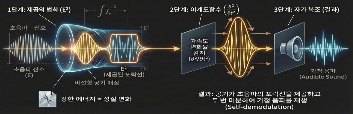
What nonlinear air does to ultrasound is, remarkably, summarized in two mathematical steps.
- The square law (E²) — Air whose properties have been altered by intense energy responds to the square of the envelope of the ultrasonic signal.
- The second derivative (∂²/∂t²) — And it produces a sound pressure proportional to the acceleration (the second derivative in time) of that squared envelope.
The result: air squares the envelope of the ultrasound, differentiates it twice, and plays back an audible wave. Nature behaves like an analog computer.
Why the square, and why exactly two derivatives? The equation of state for air does not give a perfectly straight relationship between pressure and density. Expand that deviation as a series in pressure and, after the first-order term, you get a term proportional to the square of pressure; the coefficient bundled into that term is the nonlinearity parameter β (for air, β ≈ 1.2). Since it is this second term that makes the sound, the origin of the demodulated audio is a square from the very beginning. Meanwhile, what the nonlinear term creates in the air is a distributed source, and the wave equation returns that source to sound pressure in a form differentiated twice in time. In short, the square comes from the medium's properties, and the second derivative comes from the structure of the wave equation.
Berktay's Far-Field Solution — The Engineer's Formula
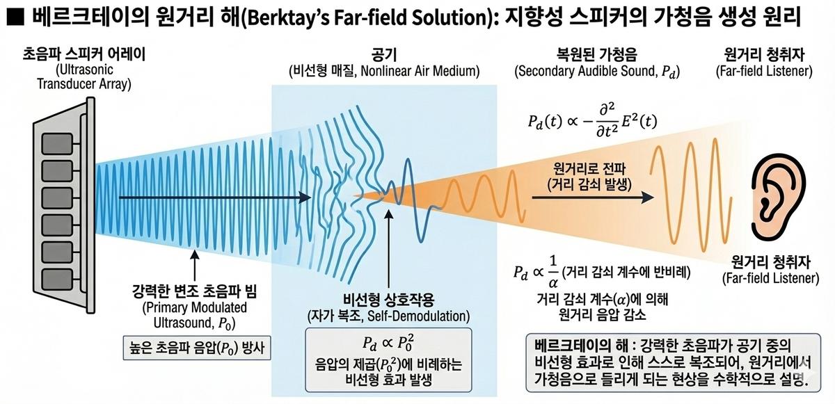
The quantification of the observation above is Berktay's far-field solution of 1965. Two conclusions are worth memorizing.
- P_d(t) ∝ −∂²/∂t² E²(t) — The audible sound pressure recovered in the far field is proportional to the second time derivative of the squared ultrasonic envelope. This formula tells you exactly what will become audible.
- P_d ∝ P₀², P_d ∝ 1/α — Audible sound is proportional to the square of the ultrasonic sound pressure and inversely proportional to the absorption coefficient α. The harder you drive the ultrasound, the louder the sound grows — quadratically; and the greater the absorption, the shorter the virtual array and the quieter the result.
Replace the proportionality signs with equalities and you get the following. For a circular source of radius a, the demodulated sound pressure on the axis at distance r is
P_d(r, t) = β · a² · P₀² / (16 · ρ₀ · c₀⁴ · α · r) × ∂²/∂t² [ E²(t − r/c₀) ]
The symbols are: β the nonlinearity parameter (1.2 for air), ρ₀ the density (1.21kg/m³), c₀ the speed of sound (343m/s), α the absorption coefficient of the carrier (Np/m), P₀ the ultrasonic pressure at the source face, and a the source radius. Two things stand out. The denominator contains the fourth power of c₀, which alone explains why air (343m/s) is so much more favorable for this conversion than water (1,500m/s). And the absorption coefficient α sits in the denominator — absorption is usually a loss, but here it sets the length of the stretch over which sound is generated, so less absorption actually means more sound.
This formula is also a design tool. The fact that you hear the square of the envelope means that loading the input signal as-is produces distortion, so the signal must be corrected (pre-processed) in advance — a topic we will meet again in the modulation and signal-processing installments, Parts 13 and 14.
Putting Numbers into the Formula
An abstract proportionality gives you no feel for the scale. Let us substitute real values. The conditions: a 100mm-diameter circular array (a = 50mm), a 40kHz carrier, an ultrasonic pressure at the source face of 130dB SPL (63.2Pa), a single tone at modulation index m = 1, and an observation distance of 1m. The absorption coefficient, from the international standard formula at 20°C, 50% relative humidity, and 1 atmosphere, is 1.32dB/m = 0.152Np/m at 40kHz. All values below are computed on an amplitude basis (converting to RMS lowers every figure by a uniform 3dB).
| Audible frequency | Demodulated pressure | Level at 1m | Per-octave difference |
|---|---|---|---|
| 200Hz | 0.0009Pa | 33.4dB | reference |
| 500Hz | 0.0058Pa | 49.3dB | +12dB/octave |
| 1kHz | 0.0233Pa | 61.3dB | +12dB |
| 2kHz | 0.0932Pa | 73.4dB | +12dB |
| 4kHz | 0.3728Pa | 85.4dB | +12dB |
Three things can be read from the table.
- Conversion efficiency is low — You radiate 130dB of ultrasound and what you get at 1kHz is 61dB. In pressure terms that is about 1/2,700. Since the sound is made not by a diaphragm but by the second-order term of the air itself, this is an unavoidable price.
- The slope is exactly 12dB per octave — The second derivative acts as the square of frequency (ω²), so 20log₁₀(2²) = 12.04dB. This term is the precise origin of the "weak bass" limitation mentioned in Part 2. Go down to 100Hz and you lose another 40dB relative to 1kHz.
- Raise the carrier by 6dB and the sound grows by 12dB — because P_d ∝ P₀². That makes carrier pressure the most effective lever for increasing output, but ultrasonic exposure guidelines and the transducer's own voltage and pressure limits set a ceiling on that lever.
The Modulation Index Is the Distortion Ratio
The formidable thing about Berktay's formula is that it lets you compute distortion by hand. Let the envelope be E(t) = 1 + m·cos(ωt) and square it:
E² = (1 + m²/2) + 2m·cos(ωt) + (m²/2)·cos(2ωt)
Differentiate twice in time and the fundamental term becomes 2m·ω² while the second-harmonic term becomes (m²/2)·(2ω)² = 2m²·ω². The ratio of the two is astonishingly simple.
second harmonic / fundamental = m
The modulation index is the second-harmonic ratio. The more signal you load on, the more distortion follows, honestly and in proportion.
| Modulation index m | Second-harmonic ratio | Level difference | Total harmonic distortion (relative to total signal) |
|---|---|---|---|
| 0.2 | 0.20 | −14.0dB | 19.6% |
| 0.5 | 0.50 | −6.0dB | 44.7% |
| 0.8 | 0.80 | −1.9dB | 62.5% |
| 1.0 | 1.00 | 0dB | 70.7% |
An ordinary loudspeaker would be criticized for 1% THD; here, full modulation yields 70%. Not because the parts are bad, but because that is what the principle dictates. So the practical remedy is not to change components but to solve the equation backwards in advance. Take the square root of the envelope you intend to send — make it E(t) = √(1 + m·s(t)) — and the moment the air squares it, the square root cancels, leaving E² = 1 + m·s(t), with the second harmonic reduced to zero in principle. That is why pre-distortion is not an option in this technology but a mandatory component.
How Long Is the Virtual Array?
For Berktay's formula to hold, the ultrasonic beam must travel like a thin, straight tube, with sound accumulating gradually along that tube. This imaginary tube is called an end-fire array. Its length is set by whichever of two values is shorter.
- The absorption length 1/α — the distance over which the carrier falls to 1/e. At 40kHz, 20°C, and 50% RH it is about 6.6m. At 25kHz it stretches to 11.9m; at 100kHz it shrinks to 2.7m.
- The Rayleigh distance R₀ = πa²/λ — the point where the near field ends and the beam begins to spread. For a 100mm diameter at 40kHz it is about 0.92m.
Comparing the two, in this configuration sound continues to be generated for a long stretch even after the beam has started to spread. That is why the virtual source of a real directional speaker is distributed over several meters in front of the speaker. It is not a metaphor when we say the sound comes not from the speaker but from a column of air.
There is also a dimensionless number that judges whether nonlinearity beats absorption. The Gol'dberg number Γ is the ratio of the shock formation distance to the absorption length; when Γ > 1, nonlinear effects appear first. Under the conditions above (40kHz, 130dB) the shock formation distance is 2.56m and Γ ≈ 2.6. Lower the carrier to 120dB and Γ falls to about 0.81, so absorption wins first — a single number telling you that unless you push the sound pressure high enough, a parametric array will not work at all.
How the Three Formulas Relate — Master, Digest, Precision Tool
- The Westervelt equation — the "master equation": It describes every nonlinear change ultrasound undergoes as it propagates. Exact, but so computationally heavy that supercomputer-class resources are often required.
- Berktay's solution — the "practical approximation": A digest of the Westervelt equation, solved simply under far-field conditions. It is the workhorse of real product design.
- The KZK equation — the "precision analysis tool": Khokhlov-Zabolotskaya-Kuznetsov. It simultaneously accounts for the big three — diffraction, absorption, and nonlinearity. This is the tool you reach for when simulating beam patterns precisely.
Stated more precisely, KZK is the Westervelt equation with a parabolic approximation applied. It assumes the beam varies rapidly along the axis and slowly across it, so transverse diffraction is handled with only the transverse part of the Laplacian. That assumption slashes the computational load, but the price is degraded accuracy for directions far off the axis (roughly beyond 20°). Berktay's solution goes one step further still, treating the beam as non-spreading and keeping only the far field on the axis.
| Aspect | Westervelt | KZK | Berktay far-field solution |
|---|---|---|---|
| Physics covered | nonlinearity, absorption, diffraction (all directions) | nonlinearity, absorption, diffraction (near the axis) | nonlinearity and absorption only |
| Core assumption | up to second-order nonlinearity | parabolic approximation | non-spreading beam plus far field |
| Valid angles | unrestricted | roughly within 20° of the axis | on-axis |
| Computational cost | very high (3D numerics) | moderate (marching along the propagation direction) | tractable by hand |
| Primary use | theoretical completeness and validation | beam pattern and near-field prediction | output and distortion estimates, pre-processing design |
The three are not rivals; they are maps at different resolutions. Quick estimates with Berktay, precise verification with KZK, theoretical completeness with Westervelt — that is how practice uses them. As numerical techniques for solving KZK in the time domain matured through the 1980s and 1990s, beam-pattern simulation became feasible even on a personal workstation.
Audible Sound Generation, Revisited in the Spectrum
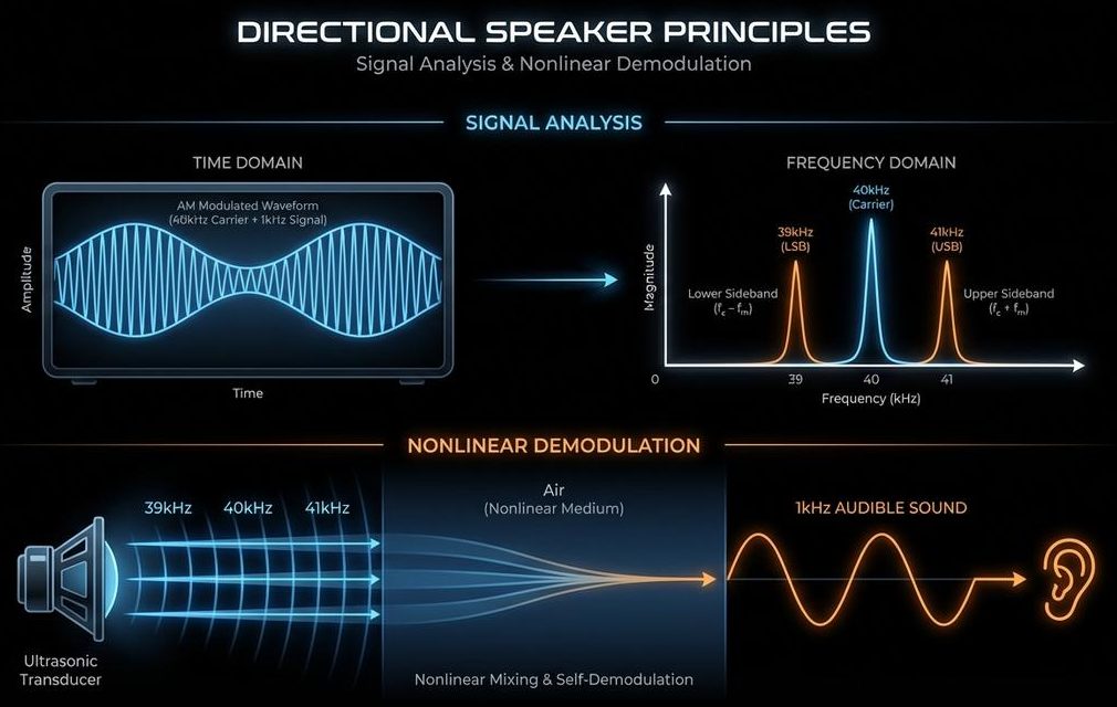
Amplitude-modulate (AM) a 1kHz voice onto a 40kHz carrier, and three peaks appear in the frequency domain — the 40kHz carrier, the lower sideband (LSB) at 39kHz, and the upper sideband (USB) at 41kHz. This is the general form of the "interaction between f1 and f2" we saw in Part 6. The air's nonlinear mixing creates the difference frequency (1kHz) between neighboring components, and that becomes the sound we hear. The time domain (squaring and differentiating the envelope) and the frequency domain (difference frequencies between sidebands) are two descriptions of the same phenomenon.
Viewed in the frequency domain, the distortion of the previous section explains itself immediately. While 40kHz and 41kHz mix to make 1kHz, 39kHz and 41kHz also mix — to make 2kHz. That 2kHz is the second harmonic. Each sideband has an amplitude of m/2 relative to the carrier, so their product scales as m²/4, while the product of carrier and sideband scales as m/2. Take the ratio and you get m once again — exactly the answer the time-domain calculation gave.
Where Berktay's Solution Fails — Limits and Common Misconceptions
- It is far-field only — the formula describes what happens after the virtual array ends. Use it to compute the pressure right in front of the speaker (inside the Rayleigh distance) and it overestimates reality. Near-field prediction is KZK's job.
- It is on-axis only — it tells you nothing about beam width or how much energy leaks sideways. It cannot answer questions such as "why is the audible sound less directional than the carrier?"
- It knows nothing of saturation — P_d ∝ P₀² does not hold indefinitely. Drive the carrier hard enough and the ultrasound itself bleeds energy into its own harmonics and saturates; beyond that point, raising the carrier no longer raises the audible output proportionally. This is especially true where the Gol'dberg number far exceeds 1.
- The misconception that "nonlinearity can create any sound" — what gets created is only the components already carried in the envelope, plus their combinations. No information appears out of nowhere.
- The misconception that this happens only in air — the theory was created for underwater sonar in the first place. Water has a larger β of 3.5, but c₀ is more than four times higher, so the c₀⁴ term makes conversion efficiency lower; in exchange, absorption is far smaller and the virtual array stretches to tens or hundreds of meters. Same formula, different constants, completely different design conclusions.
Recap
The skeleton of PAA theory fits in three sentences. The air squares the envelope of intense ultrasound and differentiates it twice to make it heard (Berktay). The complete description of the whole nonlinear process falls to the Westervelt equation. Precision simulation that embraces diffraction and absorption belongs to KZK. Add the numbers we obtained here — 12dB per octave of missing bass, a second harmonic as large as the modulation index, 12dB of audible gain per 6dB of carrier, a virtual array 6.6m long — and it becomes clear exactly where the design headroom of this technology lies. In the next part we move on to the technology that aims this sound in the direction we want — phased arrays and beamforming.
About This Series
"The Science of Directional Speakers" continues in the following order.
- What Is a Directional Speaker — A Flashlight for Sound
- Carrying Sound on Inaudible Sound — First Steps into How It Works
- Directional Speaker Use Cases — Exhibitions, Safety, Retail, and Offices
- What Is Ultrasound — Definition, Types, and Propagation
- Why Ultrasound — Generation Principles and an Application Map
- The Magic of Air Becoming a Speaker — PAA Nonlinear Acoustics
- PAA Theory Deep Dive — Berktay, Westervelt, and KZK (this installment)
- Coming up: beamforming, piezoelectric transducers, Nyquist, modulation, signal processing
This series is a blog-format adaptation of in-house lecture materials on ultrasonic directional audio technology that I researched and compiled myself. The figures are excerpted from those materials.
References
- P. J. Westervelt, "Parametric Acoustic Array," JASA 35(4), 535 (1963) : the source of the master equation — the result that nonlinear interaction of two ultrasonic beams generates a difference-frequency wave
- H. O. Berktay, "Possible exploitation of non-linear acoustics in underwater transmitting applications," JSV 2(4), 435 (1965) : the origin of the far-field solution P_d ∝ ∂²/∂t²E² used in this article
- H. O. Berktay & B. V. Smith, "End-fire array of virtual sound sources arising from the interaction of sound waves," Electron. Lett. 1(6), 202 (1965) : the origin of the virtual end-fire array concept
- S. I. Aanonsen, T. Barkve, J. N. Tjøtta & S. Tjøtta, "Distortion and harmonic generation in the nearfield of a finite amplitude sound beam," JASA 75(3), 749 (1984) : the canonical numerical treatment of the KZK equation — near-field distortion and harmonic generation
- Y.-S. Lee & M. F. Hamilton, "Time-domain modeling of pulsed finite-amplitude sound beams," JASA 97(2), 906 (1995) : the time-domain KZK method — today's standard technique for beam simulation
- Yu. Kostin & G. Panasenko, "Khokhlov–Zabolotskaya–Kuznetsov-Type Equation: Nonlinear Acoustics in Heterogeneous Media," SIAM J. Math. Anal. 40(2), 699 (2008) : the mathematical standing of KZK-type equations — derivation and validity range of the parabolic approximation
- M. F. Hamilton & D. T. Blackstock (eds.), Nonlinear Acoustics (Springer, 2024) : definitions of the nonlinearity parameter β, the shock formation distance, and the Gol'dberg number Γ — the basis for the Γ ≈ 2.6 calculation in this article
- M. Yoneyama et al., "The audio spotlight: An application of nonlinear interaction of sound waves to a new type of loudspeaker design," JASA 73(5), 1532 (1983) : the first experimental implementation of a parametric loudspeaker in air
- W.-S. Gan, J. Yang & T. Kamakura, "A review of parametric acoustic array in air," Applied Acoustics 73(12), 1211 (2012) : a review of the theory, implementation, and distortion correction of PAA in air
- H. E. Bass, L. C. Sutherland & A. J. Zuckerwar, "Atmospheric absorption of sound: Further developments," JASA 97(1), 680 (1995) : the basis (ISO 9613-1) for the 1.32dB/m (0.152Np/m) figure at 40kHz and the 6.6m absorption length used here
- Nonlinear acoustics — Wikipedia : an overview of the second-order term in the equation of state and the nonlinearity parameter β