The Science of Directional Speakers #08 — Aiming Sound: Phased Arrays and Beamforming

Parts 6 and 7 taught us how to make air produce sound (PAA). The remaining question is aiming — how do you bend the resulting beam in the direction you want? The answer is not to rotate the speaker physically. It is to manipulate time. This installment's subject is phased arrays and beamforming. And rather than describing the rules in words alone, we substitute a real 40kHz carrier and calculate where the number 4.3mm of element spacing actually comes from.

The Intuition of Ripples — Simultaneous Means Straight, Sequential Means Turned

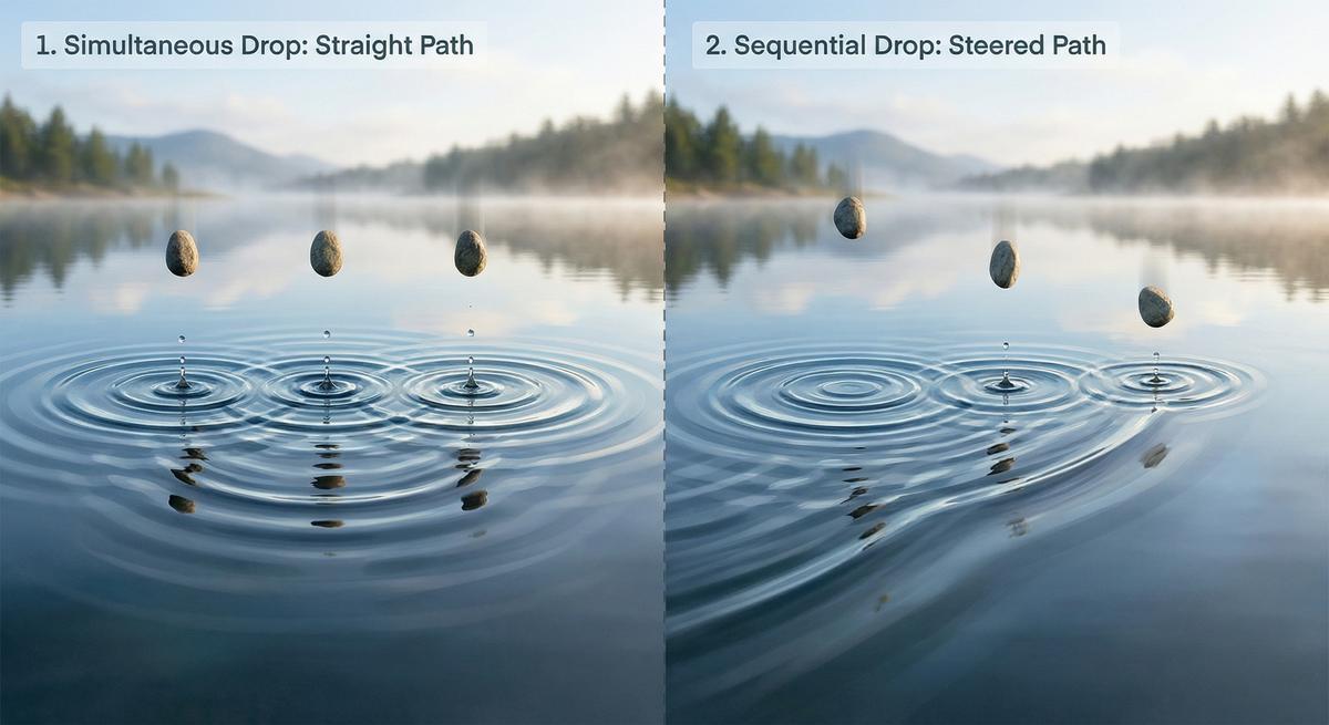
Drop three stones into a still lake simultaneously and the combined wavefront of the three ripples travels straight ahead. Now drop them in sequence, starting from the left. The earlier ripple has already spread farther by the time the later one joins, so the combined wavefront travels at an angle. The positions from which you threw the stones did not change, yet the direction of the wavefront did — and that is the whole of beamforming. Time differences create direction.

The Phased Array — Three Steps of Timing Magic

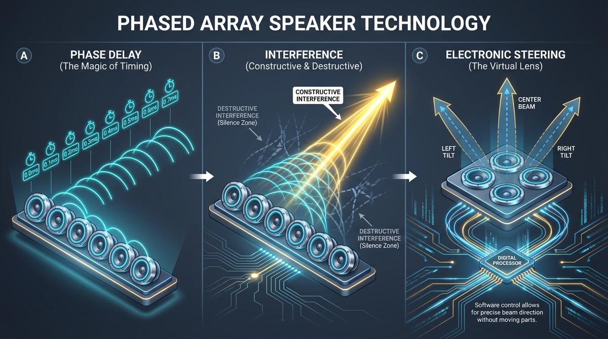
1. Phase delay — Elements arranged in a line are fired with progressively increasing time delays.
2. Interference — The waves from each element overlap; in one direction the crests meet and reinforce (constructive interference), while in the remaining directions they cancel (destructive interference — zones of silence).
3. Electronic steering — Change only the delay pattern and the beam moves left, right, or back to center. It is a "virtual lens" that changes aim in software, with no moving parts.

This is the substance of the "phase control" foreshadowed in Part 2. Incidentally, the same principle is used in radar and 5G antennas — for waves, whether sound or radio, the same mathematics applies.

Steering Angle and Phase Difference — One Equation Settles It

For waves from two neighboring elements to meet crest-to-crest in the direction θ, the difference in path length toward that direction must be exactly compensated. The path difference between two elements spaced d apart is d·sinθ, so the required time delay and phase difference are:

Δt = d·sinθ / c , Δφ = 2π·(d/λ)·sinθ [rad] = 360°·(d/λ)·sinθ

Here c is the speed of sound (343m/s) and λ the wavelength. As we saw in Part 1, the wavelength of a 40kHz carrier is λ = 343 ÷ 40,000 = 8.575mm, and one period is 25μs. Set the element spacing to half a wavelength — 4.29mm — and the formula simplifies to Δφ = 180°·sinθ. The actual values are these.

Steering angle θ	Phase difference between neighbors	Time delay	Note
0° (broadside)	0°	0μs	all elements fire together
5°	15.7°	1.09μs	—
10°	31.3°	2.17μs	—
15°	46.6°	3.24μs	—
30°	90.0°	6.25μs	a quarter of one period
45°	127.3°	8.84μs	—
60°	155.9°	10.83μs	—
90° (endfire)	180.0°	12.50μs	half a period — the theoretical limit

The important row is the last one. At d = λ/2 the phase difference required for 90° steering is exactly 180°, half a period. Since phase wraps around beyond 360°, half-wavelength spacing is the largest spacing at which every direction from 0° to 90° can be specified without phase ambiguity. That is the true identity of the d ≤ λ/2 rule that follows.

Practically, the magnitude of the delays deserves attention. Steering to 30° requires 6.25μs, so controlling that to 1° resolution needs timing resolution on the order of 0.2μs. Implemented digitally, that means a timing clock in the several-MHz range. This is why steering is done with digital signal processing rather than analog delay lines.

The Rule of Element Spacing — Spatial Aliasing and d ≤ λ/2

But you cannot lay the elements out just any way you like. If the spacing is too wide, an illusion called spatial aliasing appears.

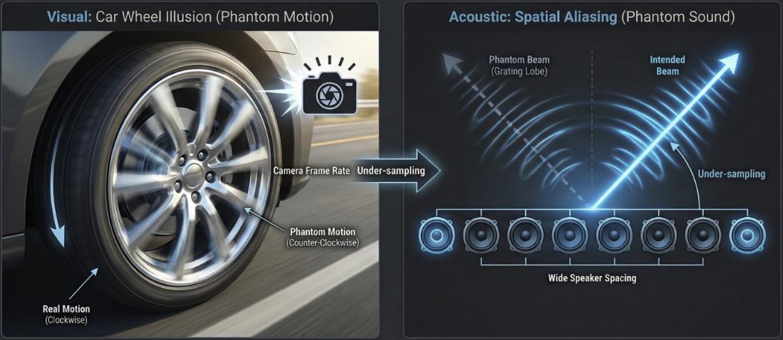
In video, a fast-spinning car wheel appears to rotate backwards because the camera's frames (sampling) cannot keep up with the wheel's rotation. A speaker array is exactly the same. If the element spacing is too wide relative to the wavelength, you have effectively sampled space too sparsely, and phantom beams appear in unintended directions.

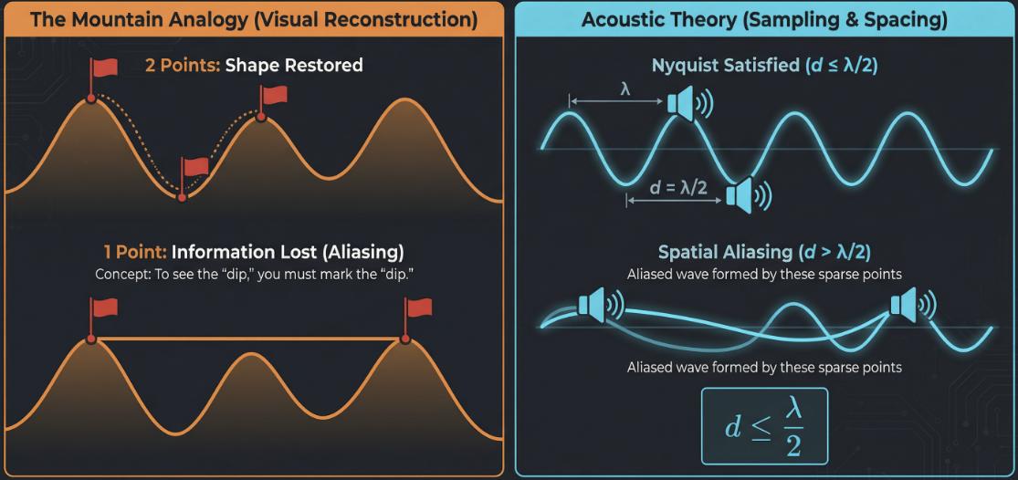
Imagine marking a mountain ridge with flags. You must plant flags in the valleys as well as on the peaks for the shape of the ridge to be recoverable. Waves are no different: the element spacing d must be at most half a wavelength (λ/2) for exactly one intended wavefront to be formed cleanly. This d ≤ λ/2 is the first rule of array design — and as you may have noticed, it is the same principle as the Nyquist theorem of digital sampling (which Part 11 addresses head-on).

Put numbers in and the rule becomes a brutally cold constraint. At 40kHz, λ = 8.575mm, so

d ≤ λ/2 = 8.575mm ÷ 2 = 4.29mm

The center-to-center distance between elements must not exceed 4.3mm — which also means the diameter of an element itself must not exceed 4.3mm. Filling a 100mm-diameter circular plate at that spacing requires about 23 elements across, roughly 420 on a square lattice, or about 490 in a hexagonal close packing. That single line explains why array designs end up with such large element counts.

Grating Lobes — The Unintended Phantom Sound Beam

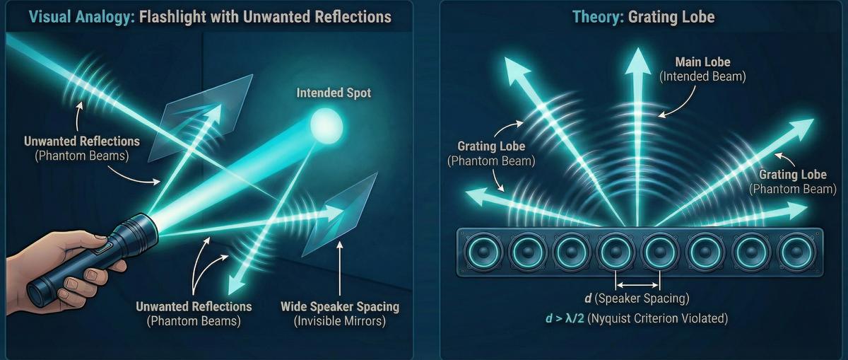
The phantom beam that appears when you break the rule (d > λ/2) even has a name — the grating lobe. It is a false beam that appears symmetrically beside the main lobe you aimed, like shining a flashlight at a wall and finding that invisible mirrors have lit up entirely the wrong places. In a directional speaker a grating lobe becomes the fatal defect of "sound the person next to you can also hear," so it must be suppressed in the spacing design.

The angle at which a grating lobe appears is calculated exactly. When the main beam is steered to θ₀, phantom beams appear at angles θ satisfying:

sinθ = sinθ₀ ± λ/d (only when |sinθ| ≤ 1 does one actually appear)

You can read off from this equation that the smaller d is, the larger λ/d becomes, until no solution exists. That is the derivation of the d ≤ λ/2 rule. To use θ₀ out to ±90° you need λ/d ≥ 2, which is exactly d ≤ λ/2. Conversely, narrow the steering range and you may widen the spacing. The condition is d/λ ≤ 1/(1 + |sinθ₀|), and at 40kHz the results are as follows.

Element spacing d	d/λ	Max steering without grating lobes	Design character
4.29mm	0.50	±90°	fully free steering
5.14mm	0.60	±41.8°	wide indoor steering
6.00mm	0.70	±25.4°	a few seats' worth
6.86mm	0.80	±14.5°	fine-trim level only
8.58mm	1.00	0° (no steering)	fixed beam only

The last row matters most. When the spacing reaches a full wavelength, even firing straight ahead sits on the boundary of a grating lobe. If you never steer at all and use a fixed forward beam, you can survive up to d < λ — but at that moment the array stops being a phased array and becomes merely several speakers glued together.

What the Element Count Decides — Beam Width and the Cost of Steering

If spacing decides the phantom beams, the element count decides the thickness of the beam. The half-power (−3dB) beam width produced by a uniformly driven linear array of length L follows this approximation:

beam width ≈ 0.886 × λ / L [rad] ≈ 50.8° × λ / L

An array filled at d = λ/2 has L = N·λ/2, so λ cancels and the beam width becomes about 101.6° ÷ N. In other words, the element count alone sets the beam width.

Elements N	Array length (4.29mm pitch)	Carrier beam width	Spot diameter at 3m
8	34.3mm	12.7°	—
16	68.6mm	6.35°	33.3cm
32	137.2mm	3.17°	16.6cm
64	274.4mm	1.59°	8.3cm
128	548.8mm	0.79°	—

This connects to the sound-zone calculation in Part 3, where a 5° beam gave a 0.26m diameter at 3m. Obtaining a beam like that requires something over twenty elements along one axis at half-wavelength pitch, meaning the array must be physically 8 to 9cm long. There is no way to narrow a beam other than adding elements — aperture is resolution.

And steering carries a price. Bend the beam by θ and the array's effective aperture shrinks by cosθ as seen from that direction, so the beam width widens by 1/cosθ. Taking N = 32 (3.17° at broadside), it becomes 3.28° at 15°, 3.66° at 30°, 4.49° at 45°, and 6.35° at 60°. Steer all the way to 60° and the beam is twice as fat as at broadside. This is why many designs limit the steering range to ±30–40°.

Side Lobes — The Price of Uniform Drive

Even if you obey every rule and eliminate grating lobes, small humps always remain beside the main beam. These are side lobes. If grating lobes are the consequence of breaking a rule, side lobes are the fate of every array with a finite aperture. As the price of the rectangular window that abruptly truncates the array (driving every element at the same amplitude), the first side lobe stops at about 13dB below the main beam. No number of added elements improves that 13dB.

The remedy is not element count but amplitude shading. Drive the edge elements more weakly so that the aperture's boundary is softened, and the side lobes drop sharply. It is the window function of signal processing applied directly to space, and representative values are these.

Drive distribution (window)	First side lobe	Main-beam width factor	Character
uniform (rectangular)	−13.3dB	1.00	maximum output, minimum beam width
Hann	−31.5dB	1.44	balanced
Hamming	−42.7dB	1.47	excellent leakage suppression
Blackman	−58.1dB	1.68	extreme suppression, large beam penalty

The table states a clear trade. Lowering side lobes by 30dB, from −13dB to −43dB, costs you a beam that is 1.5 times fatter. And since you have throttled the edge elements, total output falls as well. In a directional speaker one more factor applies — as we saw in Part 7, audible sound is proportional to the square of carrier pressure, so a side lobe that is −13dB in the carrier becomes roughly −26dB in the audible sound. The nonlinear conversion sharpens directivity one more time, one of this technology's few free gifts.

Array Geometry — Linear, Rectangular, Hexagonal

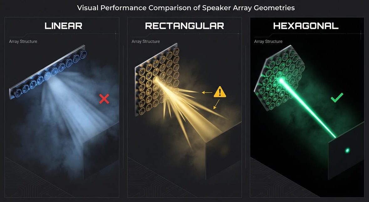
Even with the same number of elements, beam quality changes with the layout. A linear array can only narrow along one axis, so the beam spreads in a fan. A rectangular lattice narrows both axes but leaves side lobes because of the regularity of its rows and columns. A hexagonal layout packs elements most densely and produces the cleanest laser-like beam for the same area. It is the same geometry by which a honeycomb fills maximum space with minimum material.

The advantage of hexagonal packing quantifies in two ways. First, the packing fraction for circles on a plane rises from π/4 ≈ 78.5% on a square lattice to π/(2√3) ≈ 90.7% in hexagonal packing. About 1.15 times as many elements fit in the same area, and output rises accordingly. Second, the spacing at which grating lobes begin is itself more generous in a hexagonal layout. Phantom beams appear at the positions of the array lattice's reciprocal lattice, and the reciprocal lattice of a triangular (hexagonal) lattice lies 2/√3 ≈ 1.155 times farther out than that of a square lattice. By the same arithmetic, the maximum spacing permitting fully free steering (±90°) rises from 0.5λ = 4.29mm on a square lattice to 0.577λ = 4.95mm in hexagonal packing. In the 40kHz band, where shrinking elements to 4.3mm is hard, that 0.7mm of headroom is far from trivial. In addition, a square lattice concentrates phantom beams along two directions while hexagonal packing distributes them across six azimuths, lowering the chance of strong leakage in any one direction.

The Designer's Dilemma — When 4.3mm Cannot Be Met

Now for reality. A piezoelectric element that resonates at 40kHz has its physical dimensions fixed by that resonance condition (the subject of Parts 9 and 10). Widely used 40kHz ultrasonic elements come in cases about 10mm across, making 4.29mm spacing physically impossible. So what happens?

Put d = 10mm into the formula above: λ/d = 0.857, so even at broadside, sinθ = ±0.857 gives grating lobes at ±59.0°. Steer the beam by 10° and the phantom moves to −43.1°; steer by 20° and it strides in to −31.0°. The more you steer, the closer the phantom comes to the main beam.

Yet there is a reason real products work tolerably. A single element is already directional. Compute the directivity of a 10mm circular radiating face and the −3dB beam width is 52.4°, with the response at 59° already down by 14.8dB. The element factor presses down by 15dB the phantom beam that the array factor created. On top of that, audible sound is the square of the carrier, so it becomes −29.6dB — practically inaudible. The physical size of the element partially rescues the violation of the rule.

Of course this holds only near broadside; steer far and the phantom moves into the central region of the element's own directivity, where the suppression weakens sharply. To take wide-angle electronic steering seriously there is ultimately no path but making the elements smaller. That is why piezoelectric micromachined ultrasonic transducer (PMUT) arrays, whose diaphragms are fabricated directly by semiconductor processes, keep reappearing in directional-audio research — shrink an element to a few hundred micrometers and the 4.3mm rule is finally met with room to spare.

Limits and Common Misconceptions

• The misconception that "beamforming makes sound louder" — Beamforming does not create energy; it gathers it. Total radiated power merely scales with element count, and the higher on-axis pressure is the result of redirecting forward the energy that would have gone sideways.
• The misconception that "steering range is a software matter" — The upper limit on steering angle is set by element spacing, not by code. The moment d is fixed, the maximum steering angle is already decided.
• Beam-width formulas do not hold in the near field — All the approximations above assume the far field (the Fraunhofer region). Inside the Rayleigh distance computed in Part 7 (about 0.92m for a 100mm diameter at 40kHz), the beam instead propagates at roughly the aperture size, and steering does not behave as intended.
• Steering the carrier does not carry the audible directivity along unchanged — Audible sound is created by virtual sources distributed over several meters along the beam. Bending the carrier beam requires that entire column of virtual sources to tilt, so as the steering angle grows, an error opens up between the actual direction of the audible sound and the aiming direction of the carrier.
• Element-to-element variation becomes side lobes directly — Even if you design for −43dB with shading, measured side lobes will not reach that level if sensitivity and phase vary widely between elements. In designs using large element counts, element screening and per-element correction set the practical ceiling on performance.

Recap

Beamforming is the technique of creating a wavefront direction from time differences (phase), and its quality is decided by the d ≤ λ/2 spacing rule and by array geometry. Rewritten with the numbers obtained here — spacing of 4.29mm or less at 40kHz, 6.25μs of delay between neighbors for 30° steering, 32 elements and a 137mm aperture for a 3° beam, −13dB side lobes under uniform drive, and phantom beams at ±59° if you use 10mm elements — these five are the coordinates of array design. In the next part we narrow our gaze to a single element — the heart that turns electricity into sound, the piezoelectric effect.

About This Series

"The Science of Directional Speakers" continues in the following order.

1. What Is a Directional Speaker — A Flashlight for Sound
2. Carrying Sound on Inaudible Sound — First Steps into How It Works
3. Directional Speaker Use Cases — Exhibitions, Safety, Retail, and Offices
4. What Is Ultrasound — Definition, Types, and Propagation
5. Why Ultrasound — Generation Principles and an Application Map
6. The Magic of Air Becoming a Speaker — PAA Nonlinear Acoustics
7. PAA Theory Deep Dive — Berktay, Westervelt, and KZK
8. Aiming Sound — Phased Arrays and Beamforming (this installment)
9. Coming up: the piezoelectric effect, transducer design, Nyquist, modulation, signal processing

This series is a blog-format adaptation of in-house lecture materials on ultrasonic directional audio technology that I researched and compiled myself. The figures are excerpted from those materials.

References

• P. J. Westervelt, "Parametric Acoustic Array," JASA 35(4), 535 (1963) : the origin of the result that nonlinear interaction of ultrasonic beams produces difference-frequency sound — the nature of the beam being steered
• H. O. Berktay, "Possible exploitation of non-linear acoustics in underwater transmitting applications," JSV 2(4), 435 (1965) : the relation that audible sound scales with the square of carrier pressure — the basis for side lobes being suppressed twice over in the audible band
• M. Yoneyama et al., "The audio spotlight: An application of nonlinear interaction of sound waves to a new type of loudspeaker design," JASA 73(5), 1532 (1983) : the first implementation of a parametric loudspeaker in air using many ultrasonic elements arranged on a plane
• K. Aoki, T. Kamakura & Y. Kumamoto, "Parametric loudspeaker — characteristics of acoustic field and suitable modulation of carrier ultrasound," Electron. Commun. Jpn. (Part III) 74(9), 76 (1991) : measurements of the sound field and directivity of an array-type parametric loudspeaker
• F. J. Harris, "On the use of windows for harmonic analysis with the discrete Fourier transform," Proc. IEEE 66(1), 51 (1978) : the source of the side-lobe table (−13.3 / −31.5 / −42.7 / −58.1dB) and main-beam width factors used here — window functions applied directly as spatial shading
• W. Zhuang et al., "A steerable non-paraxial Gaussian beam expansion for a steerable parametric array loudspeaker," JASA 153(1), 124 (2023) : a sound-field model for steered parametric arrays — the divergence between audible beam and carrier aim at large steering angles
• S. Nakagawa et al., "Beam Steering of Portable Parametric Array Loudspeaker," APSIPA ASC 2019, 1824 : implementation and measurement of electronic steering in a compact parametric array
• G. Olszewski et al., "Steerable highly directional audio beam loudspeaker," Interspeech 2005, 137 : an early case of applying ultrasonic array steering to speech reproduction
• J. Li et al., "Piezoelectric micromachined ultrasonic transducer array for micro audio directional speaker," IEEE ICMA 2013, 450 : the PMUT array approach that shrinks elements to micrometer scale and thereby relieves the half-wavelength spacing constraint
• H. E. Bass, L. C. Sutherland & A. J. Zuckerwar, "Atmospheric absorption of sound: Further developments," JASA 97(1), 680 (1995) : atmospheric absorption of a 40kHz carrier — the upper bound on how far a steered beam actually reaches
• Phased array — Wikipedia : an overview of phase-controlled steering and the grating-lobe condition sinθ = sinθ₀ ± λ/d