The Science of Directional Speakers #10 — Ultrasonic Transducer Design: Resonance and Array Layout

Part 9 showed how a single piezoelectric element turns electricity into sound, and it left one uncomfortable number behind: producing 130dB takes 2,110V off resonance, and only 4.2V on it. This article is about how that resonance is designed. It answers two questions — how do you make one element better (structural design), and how many do you gather, and how (layout design)?

Resonance, blessing and curse — what Q decides

A piezoelectric transducer vibrates most strongly at its resonant frequency. That is the blessing. Pushing sound into a medium as light as air is fundamentally an inefficient business, and resonance multiplies the amplitude by hundreds. It is also the curse, because the sharper the resonance, the narrower the usable frequency band. The scale that measures that sharpness is the quality factor Q, and its definition is simple.

Q = resonant frequency f₀ ÷ (width Δf between the two points where amplitude falls by 3dB)

Substitute 40kHz into that one line and the first wall of the design appears immediately. Putting audio on a carrier makes the occupied band carrier ± highest audio frequency (Part 2), so the highest audio frequency you can carry is half the bandwidth.

Quality factor Q	−3dB bandwidth at 40kHz	Highest audio frequency carried	Practical use
500	80Hz	40Hz	Effectively a single tone — range sensing
200	200Hz	100Hz	On/off signalling only
40	1.0kHz	500Hz	Barely a beep
20	2.0kHz	1.0kHz	Speech, but unintelligible
10	4.0kHz	2.0kHz	Low-quality speech
5	8.0kHz	4.0kHz	Understandable speech
2.5	16.0kHz	8.0kHz	Public-announcement grade

Here is the fundamental contradiction of transducer design. The calculation in Part 9 said Q must be high for 130dB at a practical voltage; this table says Q must be low for human speech to ride along. Carrying the 8kHz needed for voice announcements demands Q of 2.5 or less, and at that point the amplitude multiplication is gone and the drive voltage climbs back into the hundreds of volts. Where you settle that contradiction is what transducer design is. Real parametric-loudspeaker elements generally sit around Q = 10 to 30 and make up the missing band with signal processing (the modulation and equalisation of Parts 12 and 13).

Thickness sets the frequency — and the 40kHz paradox

Where does the resonant frequency come from? The most basic thickness-mode resonance occurs when the plate, free on both faces, is half a wavelength thick.

t = c ÷ (2·f₀), where c is the longitudinal wave speed inside that material

Taking the thickness-mode wave speed of PZT as 4,600m/s gives the following.

Target resonant frequency	Required PZT plate thickness t = c/2f	Feasibility
5MHz	0.46mm	Medical ultrasound — routine
1MHz	2.30mm	Cleaning and machining — routine
200kHz	11.5mm	Thick, but possible
40kHz	57.5mm	Impossible — one element the size of a fist

This is the 40kHz paradox. Part 8 concluded that element diameter must be 4.29mm or less, yet a thickness-mode element at 40kHz is 57.5mm thick on its own. The mismatch exceeds a factor of ten. The lower the frequency, the thicker the piezoelectric plate, and the thicker it is, the more impossible the array becomes.

The solution is to change the mode. Instead of ringing in thickness, a thin metal disc is made to ring by bending (flexural mode). The first flexural resonance of a thin disc clamped at its edge follows, approximately:

f₀ ≈ 0.4694 × (t / a²) × √(E / (ρ(1−ν²))), with t the plate thickness and a the radius

For brass (E = 100GPa, ρ = 8,500kg/m³, ν = 0.35) the material constant is 3,662m/s. Working backwards from 40kHz gives these dimensions.

Metal disc thickness	Radius giving 40kHz	Disc diameter	Note
0.05mm	1.47mm	2.93mm	Too thin to handle
0.10mm	2.07mm	4.15mm	—
0.20mm	2.93mm	5.86mm	Practical region
0.30mm	3.59mm	7.18mm	About 10mm including the case

What was 57.5mm has become around 6mm. A flexural mode bends the plate rather than stretching it, so it resonates at a far lower frequency and lets a small part produce a low frequency. That is why the 40kHz ultrasonic elements on the market are unimorph structures — a piezoelectric plate bonded to a thin metal disc. And it is the root of the number quoted in Part 8, that "widely used 40kHz elements have a case diameter of about 10mm": add a support ring and a case to a 6mm disc and that is what you get.

Resonant structures — three ways to refine a single element

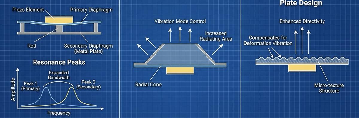
The limit of a narrow resonance is overcome not by material but by geometry. Three variations are used in practice.

• Double linked diaphragm — two diaphragms joined by a rod create two different resonant frequencies, widening the effective bandwidth between the two peaks. Overlapping two Q = 20 elements 1kHz apart, as in the table above, produces a flat stretch that a single peak cannot give.
• Radial cone — a cone mounted on the metal diaphragm shapes the vibration mode and enlarges the radiating area so that more sound goes out. It acts as an impedance transformer, moving the large displacement of a small diaphragm onto a large face.
• Micro-textured radiating plate — fine surface relief suppresses unwanted deformation modes and improves the directivity pattern. A flexural mode creates nodes and antinodes across the plate, and wherever the phase flips near a node, that becomes a side lobe.

Reading the transducer as a circuit — the BVD model

To handle design quantitatively, mechanical vibration has to be translated into a circuit. The Butterworth-Van Dyke (BVD) equivalent circuit, proposed by Van Dyke in 1928, is the standard tool. A piezoelectric resonator is represented as two branches in parallel.

clamped capacitance C₀ ∥ (motional branch: L₁ − C₁ − R₁ in series)

C₀ is the purely electrical capacitance from Part 9, while L₁, C₁ and R₁ are mechanics in translation — L₁ is the vibrating mass, C₁ the inverse of stiffness (compliance), and R₁ the loss (internal friction plus the radiation resistance that actually leaves as sound). The circuit is powerful because measurement alone recovers the physics. Read the series resonance f_s (impedance minimum) and parallel resonance f_p (impedance maximum) on an impedance analyser and the rest follows:

k_eff² = (f_p² − f_s²) ÷ f_p² , C₁ = C₀·((f_p/f_s)² − 1) , L₁ = 1 ÷ ((2πf_s)²·C₁) , R₁ = 2πf_s·L₁ ÷ Q

Let us build an example from measurable values. For an element with f_s = 40.0kHz, f_p = 41.0kHz and C₀ = 2nF:

Quantity	Expression	Value	Meaning
Effective coupling k_eff	√(1 − (f_s/f_p)²)	0.220 (k² = 4.82%)	Far below the material k of 0.7 — structural loss
Motional capacitance C₁	C₀·((f_p/f_s)²−1)	101pF	C₀/C₁ = 19.8 — the electrical side dominates twentyfold
Motional inductance L₁	1/((2πf_s)²C₁)	156mH	Equivalent mass — larger means heavier and slower
Loss resistance R₁ (Q = 20)	2πf_s·L₁/Q	1,965Ω	2.0kHz band — the floor for speech
Loss resistance R₁ (Q = 100)	2πf_s·L₁/Q	393Ω	400Hz band — tones only

The most important line is the first. The material's own k is 0.7 (the table in Part 9), yet the effective coupling measured on the finished element is 0.220. Once the piezoelectric plate moves together with a metal disc, an adhesive layer and a case, the energy stored in the non-piezoelectric parts grows by exactly that much. What the designer actually fights is not the material's theoretical figure but this structural loss. One more reading: C₀/C₁ = 19.8 means most of the electrically injected energy merely sloshes in and out of the capacitance, which is precisely why Part 9 insisted on cancelling C₀ with an inductor. More refined design uses the KLM model (1970), which treats matching layers and multilayer stacks as distributed elements, but the starting point is always these four components.

Recovering the 43dB — matching layer design

Now we settle the debt left in Part 5. The acoustic impedance of piezoceramic is about 3.3×10⁷ Rayl and that of air is 413 Rayl. When two media touch directly, the fraction of acoustic energy transmitted is

T = 4·Z₁·Z₂ ÷ (Z₁ + Z₂)² = 4 × 3.3×10⁷ × 413 ÷ (3.3×10⁷ + 413)² = 5.01×10⁻⁵

That is 0.005%, or −43.0dB. Fewer than one part in ten thousand gets out. This is what the −43dB of Part 5 actually was. The remedy uses the same principle as an anti-reflection coating in optics — insert a quarter-wave matching layer of intermediate impedance. When the layer is exactly λ/4 thick as measured inside itself, the waves reflected from its front and back faces are half a cycle apart and cancel, maximising transmission. The ideal impedance is the geometric mean of the two.

Z_m = √(Z_piezo × Z_air) = √(3.3×10⁷ × 413) = 116,700 Rayl (0.117 MRayl)

The trouble is that this value is absurdly low. Water is 1.5 MRayl and rubber about 1 MRayl, so the layer has to be ten times lighter than rubber. Here is how much can be recovered with materials that actually exist (single layer, at the centre frequency).

Matching layer material (example)	Impedance Z_m	Transmission T	dB	Improvement over none
None (direct radiation)	—	0.005%	−43.0dB	reference
Epoxy with hollow microspheres	1.50 MRayl	2.39%	−16.2dB	+26.8dB
Silicone rubber	1.00 MRayl	5.31%	−12.8dB	+30.2dB
Porous polymer	0.30 MRayl	45.7%	−3.4dB	+39.6dB
Ideal matching layer (theory)	0.117 MRayl	100%	0dB	+43.0dB

Getting down to just 0.3 MRayl already yields −3.4dB, meaning nearly half gets through. An improvement approaching 40dB means a single matching layer changes transducer efficiency by a factor of ten thousand. But reaching such a low impedance demands an extremely light material — aerogels, foams, hollow-microsphere fillers — and such materials are usually lossy, moisture-sensitive and mechanically fragile. Practical designs therefore step the impedance down in stages. The binomial solution gives 0.766 and 0.018 MRayl for two layers, and 1.96 / 0.117 / 0.0069 MRayl for three — the fact that each added layer demands an even lighter final layer captures the fundamental difficulty of this technology.

Thickness is no easier. Since λ/4 is computed with the layer's own sound speed, a porous layer at 400m/s needs 2.5mm at 40kHz and a foam at 150m/s needs 0.94mm. With an element only 6mm across, a 2.5mm matching layer means half the part is matching layer. And because the quarter-wave condition is exact at one frequency only, adding a matching layer narrows the bandwidth once again.

Backing — buying bandwidth with output

What sits behind the piezoelectric plate is also a design decision. With air behind it, almost no energy leaves backwards, so efficiency is maximal, but the vibration rings on: high Q, narrow band. Attach an absorbing backing such as tungsten-loaded epoxy and the vibration dies quickly, lowering Q and widening the band, but that much energy escapes rearward. At the extreme, matching the backing impedance to the ceramic sends half the energy backwards, a −3dB price. Kossoff's classic 1966 study laid out exactly this trade. Pulse transducers for medicine and non-destructive testing live on short pulses and use thick backing; a directional loudspeaker aims for maximum continuous-wave output and uses almost none. It is a textbook case of the same component being designed in opposite directions for different uses.

Horns — amplifying displacement with geometry

Another classical technique is the horn. Attach a metal bar of decreasing cross-section to the resonator and conservation of energy raises the vibration amplitude at the narrow end. For a stepped horn the theoretical amplitude gain equals the area ratio: a 2:1 diameter ratio gives 4 times (+12.0dB) and 3:1 gives 9 times (+19.1dB). The gain, however, comes from large amplitude on a small face, so the radiating area shrinks and directivity actually gets worse (the wavelength-to-aperture ratio of Part 1). Horns are therefore standard in high-power ultrasonic machining, while a directional loudspeaker, which needs a wide aperture, chooses the opposite — the radial cone that enlarges the area. Same physics, opposite direction.

Why gather them into an array — gains and costs

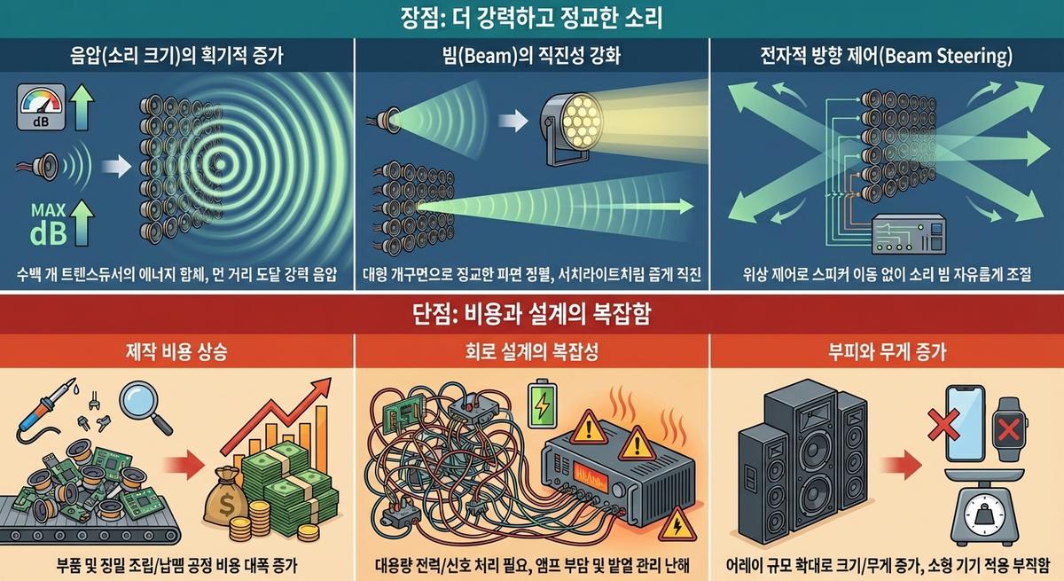
One element does not make a directional loudspeaker. As calculated above, a 40kHz element is 6 to 10mm across, and by the wavelength-to-aperture ratio of Part 1 such an aperture is nearly omnidirectional against an 8.6mm wavelength. Arraying hundreds brings clear gains and clear costs.

• Gains — (1) the combined energy of hundreds of elements, the key to crossing the threshold where nonlinear effects appear; (2) a well-formed wavefront and straight propagation from a large aperture (D ≫ λ); (3) the phase-controlled beam steering of Part 8.
• Costs — (1) a steep rise in parts, assembly and soldering cost; (2) circuit complexity entangling high-current drive, signal processing and thermal management (recall the reactive-current table of Part 9 — 400 elements in parallel is 0.8μF); (3) size and weight proportional to the array.

The power of numbers — 20log(N) and hexagonal rings

How much does on-axis pressure rise when N elements are gathered? If every element rings in phase, the pressure amplitude on axis is simply N times greater. Note that it is the amplitude, not the energy, that scales with N.

on-axis pressure gain = 20·log₁₀(N) [dB] , total radiated power increase = 10·log₁₀(N) [dB]

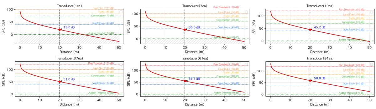
The difference between the two, 10·log₁₀(N), is the directivity gain — the share of energy redirected from the sides to the front. (It is the equation behind Part 8's remark that beamforming gathers energy rather than creating it.) Taking a single element that produces 19.6dB at 20m, and noting that hexagonal close packing grows as 3n(n+1)+1 for n rings:

Hexagonal rings	Elements N	On-axis gain 20log(N)	SPL at 20m	Array width at 10mm pitch
0	1	0dB	19.6dB	10mm
1	7	+16.9dB	36.5dB	30mm
2	19	+25.6dB	45.2dB	50mm
3	37	+31.4dB	51.0dB	70mm
5	91	+39.2dB	58.8dB	110mm
7	169	+44.6dB	64.2dB	150mm

At 20m, a single element gives 19.6dB — effectively inaudible. Nineteen elements reach 45.2dB, above the level of a quiet room, and ninety-one give 58.8dB, approaching the carrying power of ordinary conversation at 70dB. The "clear sound tens of metres away" promised in Part 1 is a number that only holds with enough elements in the right geometry. The last column deserves equal attention: ninety-one elements on a 10mm hexagonal pitch make an array 110mm wide. As calculated in Part 8, only an aperture of that order narrows the carrier beam, and it also pushes the Rayleigh distance of Part 7 out towards a metre. Sound pressure and directivity are decided by the same dimension at the same time.

One caveat: 20log(N) is an ideal ceiling. If element resonant frequencies scatter by ±1%, the phases no longer align, the summation is imperfect, and the gain is trimmed accordingly. That is why binning elements is effectively a mandatory process step in large arrays.

The designer's synthesis — how one 40kHz transducer comes to be

Lay the decisions so far in order and you have the actual design flow.

• 1. Choose the mode — thickness resonance at 40kHz is 57.5mm and therefore impossible; go with the flexural mode of a thin metal plate.
• 2. Fix the dimensions — 0.2mm brass plate, radius 2.93mm (diameter 5.9mm), about 10mm including the case.
• 3. Set the Q target — work backwards from the audio band required. 2kHz speech needs Q ≤ 10; in practice settle at Q = 10 to 30 and cover the shortfall in signal processing.
• 4. Treat the front and back faces — recover the −43dB into the −3 to −16dB range with a matching layer, budgeting the further band narrowing against step 3, and keep backing minimal since continuous-wave output is the goal, while securing a thermal path.
• 5. Match electrically and array — cancel C₀ with an inductor (the table in Part 9), then derive N from the target SPL (20log N) and the aperture from the target beamwidth (Part 8); the larger of the two sets the array size.

As the sequence shows, this design has almost no free variables. Choosing 40kHz as the carrier fixes the element size; the element size then collides with the spacing rule of Part 8; and the bandwidth requirement collides with output through Q.

Limits and common misconceptions

• "A good transducer is a sensitive one." In a parametric loudspeaker, bandwidth and distortion decide audio quality more than sensitivity. Harmonics generated by element nonlinearity are demodulated as noise, indistinguishable from the nonlinearity of the air.
• "A matching layer is always a win." A matching layer buys efficiency at the cost of bandwidth, and the internal loss of the layer material eats part of the gain back. The lighter and lossier the material, the larger that offset.
• "Thicker backing is better." Backing is a trade that sells output to buy bandwidth. For continuous-wave use it is usually a loss.
• More elements do not improve sound quality. Count changes sound pressure and beamwidth; bandwidth and distortion remain those of a single element. A hundred elements still cannot produce a frequency that none of them can.
• No two elements are identical. Unit-to-unit spread in resonant frequency and sensitivity undermines both the ideal 20log(N) summation and the side-lobe design of Part 8 at once. The practical performance ceiling of a large array is usually set right here.

Summary

Transducer design has two layers. At the element layer you trade bandwidth against efficiency through mode (thickness versus flexural), Q, matching layers and backing; at the system layer you buy sound pressure and aiming ability at the price of cost, complexity and size. Restated in this article's numbers: thickness resonance at 40kHz would be 57.5mm and is impossible; the flexural route gives a 0.2mm plate 5.9mm across; unmatched radiation is −43dB while a 0.3 MRayl layer brings it to −3.4dB; carrying 8kHz speech demands Q ≤ 2.5; and ninety-one elements in a hexagon give 58.8dB at 20m. That closes the hardware story — from the next article we move into the digital world. The first gate is the rule for turning analogue sound into numbers, the Nyquist theorem.

Series guide

"The Science of Directional Loudspeakers" runs in the following order.

1. What is a directional loudspeaker — a flashlight for sound
2. Carrying sound on sound you cannot hear — first steps in operating principle
3. Applications — exhibitions, safety, retail, offices
4. What is ultrasound — definitions, types, propagation
5. Why ultrasound — generation principles and application map
6. The magic of air becoming a loudspeaker — PAA nonlinear acoustics
7. PAA theory in depth — Berktay, Westervelt, KZK
8. Aiming sound — phased arrays and beamforming
9. The piezoelectric effect — the moment electricity becomes sound
10. Ultrasonic transducer design — resonance and layout (this article)
11. Coming next: Nyquist, modulation, signal processing

This series is a blog adaptation of self-produced lecture material researched and compiled on ultrasonic directional audio technology. The figures are excerpted from that material.

References

• K. S. Van Dyke, "The Piezo-Electric Resonator and Its Equivalent Network," Proc. IRE 16(6), 742 (1928) : the original paper behind the BVD equivalent circuit (C₀ ∥ L₁C₁R₁) used here — the standard for translating mechanical vibration into a circuit
• R. Krimholtz, D. A. Leedom & G. L. Matthaei, "New equivalent circuits for elementary piezoelectric transducers," Electronics Letters 6(13), 398 (1970) : the KLM model, treating matching layers and backing as distributed elements — the standard tool for multilayer transducer design
• G. Kossoff, "The Effects of Backing and Matching on the Performance of Piezoelectric Ceramic Transducers," IEEE Trans. Sonics Ultrason. 13(1), 20 (1966) : the classic account of how backing and matching trade sensitivity against bandwidth — the basis of the backing section
• C. S. Desilets, J. D. Fraser & G. S. Kino, "The design of efficient broad-band piezoelectric transducers," IEEE Trans. Sonics Ultrason. 25(3), 115 (1978) : impedance design theory for multiple quarter-wave matching layers — the lineage of the two- and three-layer values quoted here
• T. E. Gómez Álvarez-Arenas, "Acoustic impedance matching of piezoelectric transducers to the air," IEEE TUFFC 51(5), 624 (2004) : the ultra-low-impedance materials and porous layers that air matching demands — the basis of the matching-layer table
• B. Jaffe, R. S. Roth & S. Marzullo, "Piezoelectric Properties of Lead Zirconate-Lead Titanate Solid-Solution Ceramics," J. Appl. Phys. 25(6), 809 (1954) : the material starting point for the PZT used in the thickness-resonance and impedance calculations here
• IEEE Std 176-1987, IEEE Standard on Piezoelectricity : the standard definition of the measurement convention for effective coupling k_eff from series and parallel resonance
• M. Yoneyama et al., "The audio spotlight: An application of nonlinear interaction of sound waves to a new type of loudspeaker design," JASA 73(5), 1532 (1983) : the first parametric loudspeaker built from many ultrasonic elements on a plane — the archetype of array design
• K. Aoki, T. Kamakura & Y. Kumamoto, "Parametric loudspeaker — characteristics of acoustic field and suitable modulation of carrier ultrasound," Electron. Commun. Jpn. (Part III) 74(9), 76 (1991) : measured field and directivity characteristics of array-type parametric loudspeakers
• C. Shi & Y. Kajikawa, "Effect of the ultrasonic emitter on the distortion performance of the parametric array loudspeaker," Applied Acoustics 112, 108 (2016) : measurements of how a transducer's narrow band and nonlinearity appear as reproduction distortion — the basis of the limits section
• J. Li et al., "Piezoelectric micromachined ultrasonic transducer array for micro audio directional speaker," IEEE ICMA 2013, 450 : the PMUT approach, making flexural membranes by semiconductor processing to break the element-size constraint
• H. E. Bass, L. C. Sutherland & A. J. Zuckerwar, "Atmospheric absorption of sound: Further developments," JASA 97(1), 680 (1995) : the basis of the 40kHz atmospheric absorption coefficient used in the 20m reach calculation