The Science of Directional Speakers #11 — The Nyquist Theorem: The Starting Point of Digital Sound

Through Part 10 we completed the hardware of a directional speaker. The stage now moves to the digital domain. In a real product, sound travels through analog → ADC (conversion to numbers) → digital processing → DAC (back to analog) → filter. Standing at the very start of that journey is today's subject — the Nyquist–Shannon sampling theorem.

In ordinary audio gear this theorem is usually summarized in one line: "44.1kHz is enough." But the signal we handle is a 40kHz ultrasonic carrier. The moment you must synthesize a frequency more than twice the upper limit of hearing, the theorem stops being a summary and becomes the equation that fixes your design specification. What sampling rate is required, how many poles the filter in front of it needs, how many bits are necessary, how much latency appears — all of it branches out from this single line.

Two Axes That Turn Sound into Numbers — Sample Rate and Bit Depth

Moving a continuous analog waveform into the digital domain means slicing it in two directions.

• Sample rate — the time axis. It sets how many times per second the waveform's value is recorded. CD audio records 44,100 times per second (44.1kHz).
• Bit depth — the amplitude axis. It sets how fine a scale each recorded value is placed on. Sixteen bits gives 65,536 steps.

The two axes behave very differently. Bit depth is a question of "how precisely," so a shortage merely raises the noise floor, and noise is a component added on top of the original signal, which means it can be managed to some extent later. But if the sample rate is insufficient, the sound itself turns into a different sound. The disguised signal sits inside the same band as the original, so once it has been recorded that way, no amount of post-processing can separate it. The difference between a recoverable mistake and an unrecoverable one — that is why the time-axis rule comes first.

Sample Too Sparsely and Ghosts Appear — Aliasing

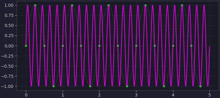
If samples are taken too sparsely, the waveform reconstructed by connecting those points becomes a false low frequency that bears no relation to the original. This ghost signal is aliasing. We see it in everyday life — the illusion of an aircraft propeller in a video appearing to rotate slowly backwards is exactly the same phenomenon. The camera's frame rate (time sampling) cannot keep up with the propeller's rotation.

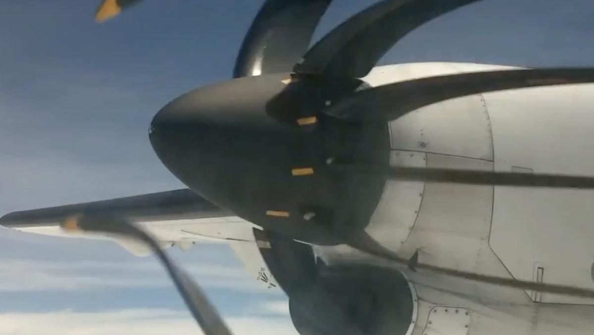
Where the ghost lands can be calculated exactly. Sampling an input frequency f at rate f_s produces a folded frequency equal to the distance from f to the nearest integer multiple of f_s.

f_alias = | f − round(f ÷ f_s) × f_s |

Substituting the frequencies actually encountered in a directional speaker makes the danger of a wrong sample rate immediately visible. Every value below was computed directly from that expression, and the bold cells are the cases where the ghost lands inside the audible band (20Hz–20kHz) and is genuinely heard.

Input frequency	Sampled at 48kHz	Sampled at 96kHz	Sampled at 192kHz	Sampled at 384kHz
20kHz (top of hearing)	20kHz correct	20kHz correct	20kHz correct	20kHz correct
40kHz (carrier)	8kHz ghost	40kHz correct	40kHz correct	40kHz correct
60kHz (edge of upper sideband)	12kHz ghost	36kHz ghost	60kHz correct	60kHz correct
80kHz (2nd harmonic of carrier)	16kHz ghost	16kHz ghost	80kHz correct	80kHz correct
100kHz (switching residue)	4kHz ghost	4kHz ghost	92kHz ghost	100kHz correct
120kHz (switching residue)	24kHz ghost	24kHz ghost	72kHz ghost	120kHz correct

The second row is the most alarming cell in this table. Sample a 40kHz carrier at the 48kHz of a common audio interface and the carrier vanishes, leaving a clearly audible 8kHz tone. A signal that was supposed to be inaudible relocates into the very middle of the band where hearing is most sensitive. From the third row the failure becomes subtler — 96kHz captures the 40kHz carrier itself correctly, but the sidebands beside it (60kHz) and the harmonic (80kHz) fold back into the signal band. In other words, you cannot choose a sample rate by looking at the carrier alone.

The Nyquist–Shannon Theorem — The Rule of Two

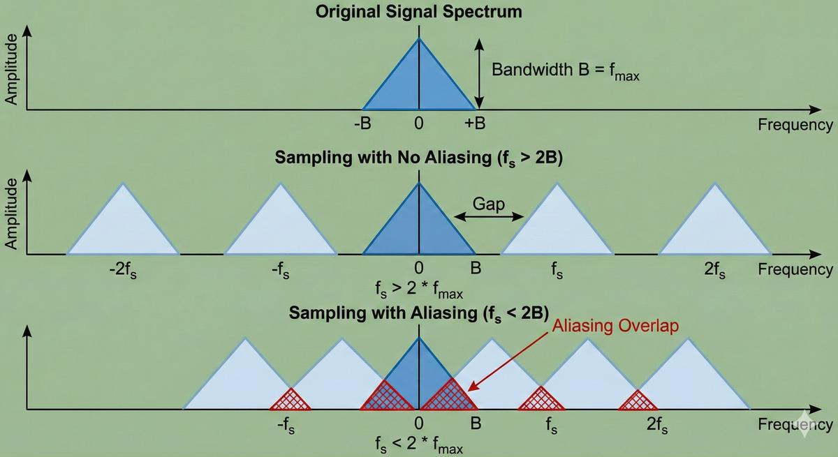
So how densely must we sample to be safe? The theorem's answer is unambiguous — sample faster than twice the highest frequency in the signal (f_s > 2·f_max). The frequency domain shows why. Sampling replicates copies of the original spectrum at intervals of f_s. If f_s obeys the rule of two, a gap remains between the copies and the original can be cleanly cut out; if the rule is broken, the copies overlap and the original can no longer be recovered. This is also why CD uses 44.1kHz — twice the 20kHz audible limit (40kHz), plus a margin for the filter.

Two names are attached to this rule. In a 1928 paper on telegraph transmission theory, a limit was presented: a channel of bandwidth B can carry 2B independent pulses per second. That was a question about the capacity of a transmission line, not about converting sound into numbers. The result was formalized in the shape of complete reconstruction of the original signal from its samples in a 1949 paper, and there the form we use today appears — interpolating the samples with sinc functions restores the original band-limited signal exactly. A theorem born in the language of communications took some two decades to become the common foundation of audio, imaging, and instrumentation.

Two caveats must be remembered in practice. First, what the theorem demands is that the signal be perfectly band-limited. Real signals always carry out-of-band components and noise, so a filter is mandatory ahead of the sampler. Second, the inequality does not include equality. If f_s is set to exactly 2·f_max, a component sitting precisely at the Nyquist frequency may, depending on its phase, be sampled at amplitude zero. Sampling 40kHz at exactly 80kHz gives two points per cycle, and if those two points always land on the zero crossings, every recorded value is zero. The rule is "more than twice," not "at least twice," and in practice the excess is made generous.

Time and Space Are the Same Mathematics — The Link to Part 8

You will recall from Part 8 that array element spacing must satisfy d ≤ λ/2. At the time we merely noted that this was "the same principle as the Nyquist theorem in digital sampling," and now we can verify that claim precisely. The two rules are not an analogy; they are the same equation with the variable names changed.

An array samples a continuous wavefront spatially, at the element positions. If the time sampling rate is samples per second, the spatial sampling rate is samples per metre — that is, 1/d. And what corresponds to the highest temporal frequency f_max is the highest spatial frequency 1/λ. Substituting directly into the rule of two gives

1/d > 2 × (1/λ) ⟹ d < λ/2

The first rule of Part 8 has been derived from the sampling theorem in a single line. The correspondences run as follows — sample interval Δt ↔ element spacing d, sample rate f_s ↔ 1/d, Nyquist frequency f_s/2 ↔ 1/(2d), aliasing ↔ grating lobes, anti-aliasing filter ↔ element directivity. That last pair is especially interesting. On the time axis an analog filter removes out-of-band components in advance; on the spatial axis the directivity pattern of each individual element suppresses components arriving from large angles and thereby weakens grating lobes. Limiting element diameter to λ/2 or less in Part 8 was, in effect, anti-aliasing design in the spatial domain.

The Anti-Aliasing Filter — The Real Cost Is the Transition Band

As noted, an anti-aliasing filter that removes components above the Nyquist frequency always sits ahead of the sampler. The difficulty is that an ideal wall cannot be built. A real filter descends gradually across a transition band from the passband edge (f_p) to the start of the stopband (f_stop). And where the stopband must begin is fixed — to prevent anything folding into the passband, f_stop = f_s − f_p.

The required attenuation is fixed too. The folded component must be smaller than the quantization noise to be harmless, so for a 16-bit system the benchmark is the roughly 98dB we calculate later. An analog filter attenuates 6dB per octave per pole, so the number of poles needed is 98dB divided by the width of the transition band in octaves. Below are those results.

Condition	Passband edge	Stopband start	Transition width (octaves)	Poles needed for 98dB
CD audio (44.1kHz)	20kHz	24.1kHz	0.27	about 60 poles (practically impossible)
48kHz audio	20kHz	28kHz	0.49	about 34 poles
192kHz, audio band only	20kHz	172kHz	3.10	about 5.2 poles
192kHz, carrier band	60kHz	132kHz	1.14	about 14.3 poles
384kHz, carrier band	60kHz	324kHz	2.43	about 6.7 poles

The first row is the wall that early digital audio ran into in the 1970s and 80s. Staying flat to 20kHz and then falling 98dB by 24.1kHz requires an analog filter of more than 60 poles, which cannot be built — and even if it could, its phase response inside the passband would be badly distorted. Economize on sample rate and the bill arrives at the analog filter — that is the conclusion of the table. Conversely, raising the sample rate widens the transition band and the filter gets dramatically easier. At 192kHz, handling only the audio band, an ordinary 5-pole filter suffices.

Oversampling — Moving the Filter from Analog into Software

The strategy built on that observation is oversampling. The idea is simple: sample far faster than necessary so the analog filter has almost nothing to do, perform the genuinely sharp cutoff later, in a digital filter, then drop the rate to the value you actually need (decimation). It trades a characteristic that is hard to build in the analog domain for one built in the digital domain, and since a digital filter is defined by its coefficients, it has no component tolerance and no temperature drift.

A bonus follows. The total quantization noise power is fixed regardless of sample rate, but oversampling spreads that total across a wider frequency range. The noise remaining inside the band of interest falls accordingly, and the gain is 10·log₁₀(OSR) dB — 6dB, that is one bit, for every factor of four. You buy one bit by quadrupling the sample rate, and adding noise shaping, which actively pushes noise out of band, makes the exchange rate far more favourable. This is the principle by which a sigma-delta converter achieves 24-bit-class performance from a quantizer of nearly one bit.

• 2× oversampling — 3.0dB gain, 0.5 bit
• 4× — 6.0dB, 1 bit
• 8× — 9.0dB, 1.5 bits
• 16× — 12.0dB, 2 bits

In a directional speaker this strategy matters most on the output side. The reconstruction filter after the DAC faces the same problem as the anti-aliasing filter, and to that is added the attenuation of the staircase output itself (zero-order hold). Zero-order hold rolls off high frequencies with a sinc shape relative to f_s; computing what a 40kHz carrier suffers at 192kHz gives 0.63dB. The same calculation for 20kHz at 48kHz gives 2.64dB — more than four times as much. Simply raising the sample rate reduces carrier amplitude loss on its own, and the remaining 0.63dB can be pre-compensated in the digital filter.

Precision on the Amplitude Axis — 6.02N + 1.76

Now the second axis. Quantization rounds a continuous value to the nearest step, and the error discarded in that act is quantization noise. The analysis treating this error as noise distributed uniformly across one step width was set out in 1948, and on that basis the signal-to-noise ratio for a full-scale sine wave follows in one line.

SNR = 6.02 × N + 1.76 [dB] (N = number of bits)

The coefficient 6.02 says that each bit halves the amplitude step (20·log₁₀2 = 6.02dB), and 1.76 is the constant arising from the ratio between the RMS value of a sine wave and that of uniformly distributed noise. One bit equals exactly 6dB — this conversion factor is the basic unit of audio design.

Bits	Quantization steps	Theoretical SNR	One step at 2V full scale	Typical use
8-bit	256	49.9dB	7.81mV	noise clearly audible
12-bit	4,096	74.0dB	488µV	control and instrumentation
16-bit	65,536	98.1dB	30.5µV	the distribution-format benchmark
20-bit	1,048,576	122.2dB	1.91µV	high-grade converters
24-bit	16,777,216	146.2dB	0.12µV	internal processing headroom

The last row is frequently misunderstood. The 146dB of 24 bits is not a figure anyone actually obtains; the thermal noise of resistors at room temperature alone buries the digits below it. Twenty-four bits are used not to hear 146dB but to secure headroom to squander during processing. Lowering gain and raising it again, passing through several filter stages, repeating modulation arithmetic — all of it consumes the lower bits. Performing internal processing at generous word length and reducing only the output to 16 bits is the standard arrangement.

A directional speaker adds one more concern. If the instant at which samples are taken jitters (aperture jitter), that alone becomes noise, and the limit is −20·log₁₀(2π·f·t_j). Since the signal frequency f sits in the argument, higher frequencies are hurt more by the same jitter. With 1 nanosecond of jitter, 20kHz still holds 78dB while 40kHz drops to 72dB; to preserve 16-bit performance (98dB) at 40kHz, jitter must be kept below about 100 picoseconds (which yields 92dB by the same formula). This is why systems handling an ultrasonic carrier are unusually fussy about their clock circuits.

Sampling in a Directional Speaker — Handling 40kHz

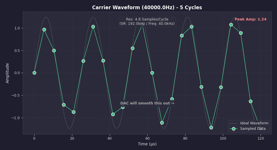
Here the peculiarity of the directional speaker emerges. Ordinary audio equipment only needs to handle up to 20kHz, but we must synthesize a 40kHz ultrasonic carrier digitally. The Nyquist rule sets a floor of 80kHz — in practice a margin is added and 192kHz sampling is used. That secures 4.8 samples per cycle of the 40kHz carrier, and after DAC interpolation the waveform is restored smoothly. An ordinary sound card (44.1/48kHz) cannot even generate the carrier — which is why the signal-processing hardware of a directional speaker differs from audio equipment.

That said, "80kHz is enough" holds only if you look at the carrier alone. What must actually be emitted is the modulated signal, and amplitude-modulating audio up to 20kHz onto a 40kHz carrier spreads the spectrum from 20kHz (edge of the lower sideband) to 60kHz (edge of the upper sideband). Applying the square-root preprocessing covered in Parts 12 and 13 widens it further. If the highest frequency is 60kHz, the Nyquist minimum is 120kHz, and securing a transition band demands more than that. Weighing the candidates gives the following.

Sample rate	Nyquist frequency	Samples per 40kHz cycle	Covers up to 60kHz?	Verdict
48kHz	24kHz	1.2	no	carrier folds down to 8kHz
96kHz	48kHz	2.4	no	carrier survives but sidebands fold
192kHz	96kHz	4.8	yes (36kHz margin)	the standard choice
384kHz	192kHz	9.6	yes (132kHz margin)	harmonics manageable, twice the computation

The table shows why 192kHz is the answer. Subtracting the 60kHz signal ceiling from the 96kHz Nyquist frequency leaves a 36kHz margin, and that width is precisely the runway on which the anti-aliasing and reconstruction filters descend. As computed in the filter table, this condition corresponds to roughly 14 poles — a level at which most of the work can be done digitally and the analog side finished with a single gentle low-pass. Choosing 384kHz instead lets you manage even the second harmonic of the carrier (80kHz) without distortion, but for the same filter length the computation and power consumption double. Choosing a sample rate is a trade between filter difficulty and computational cost, and for a 40kHz carrier that balance point sits near 192kHz.

Block Size Sets the Latency — The Real-Time Condition

Sample rate bears directly on latency as well. Digital signal processing usually operates not on one sample at a time but on blocks of gathered samples. Waiting for a block to fill becomes latency directly, and its value follows from a single division.

buffer latency = block length (samples) ÷ sample rate

For the same block length, a higher sample rate means lower latency. Below is that calculation; the right-hand column converts the time into the distance sound travels through air (speed of sound 343m/s). Reading latency as "equivalent to moving the speaker back by how many centimetres" makes it intuitive.

Block length	Latency at 48kHz	Latency at 192kHz	192kHz latency as distance
32 samples	0.67ms	0.17ms	5.7cm
64 samples	1.33ms	0.33ms	11.4cm
128 samples	2.67ms	0.67ms	22.9cm
256 samples	5.33ms	1.33ms	45.7cm
512 samples	10.67ms	2.67ms	91.5cm
1024 samples	21.33ms	5.33ms	182.9cm

Shorten the block and latency falls, but the fixed cost attached to every block (function calls, filter-state updates, interrupt handling) takes a larger share and computational efficiency drops. Lengthen it and efficiency improves while latency grows. At 192kHz, 256 samples is 1.33ms — the time sound takes to travel 46cm, which in most installations disappears inside the propagation delay to the listener. The full latency budget must add the filter delays as well, and that accounting is revisited item by item in Part 14.

Limits and Common Misconceptions

• "Sampling makes staircases, so it differs from the original." The most common misconception. The staircase between samples is not a property of sampling but merely the shape of the DAC output before the reconstruction filter. If the band-limiting condition was respected, the samples contain every bit of the original signal's information, and sinc interpolation restores the waveform exactly. The staircase is erased by the final filter.
• "Higher sample rates are always better." They are not free. Computation, memory, and power scale with the rate, and the widened band admits more out-of-band noise and jitter influence. Once the signal ceiling is fixed, the required rate is something you calculate, not something you raise indefinitely.
• "More bits make the sound louder." Bit depth sets not maximum volume but the distance between the quietest and loudest sound (dynamic range). Volume is the amplifier's business.
• "Aliasing can be filtered out afterwards." It cannot. Folded components sit inside the signal band and are indistinguishable from genuine ones. That is why the anti-aliasing filter must be ahead of the sampler; no digital filter, however good, can separate what has already been mixed.
• "Obey the theorem and everything is perfect." The theorem describes ideal conditions: a perfectly band-limited signal, sinc interpolation of infinite length, a jitter-free clock, error-free quantization. None of the four exists. The theorem tells you the line you must not cross; the quality inside that line is decided by filter, clock, and bit-depth design.

Summary

Digital sound is recorded by samples per second (rate) and steps of scale (depth), and sampling must exceed twice the highest frequency for the original to be preserved. Break the rule and ghosts appear on the time axis (aliasing) and on the spatial axis (grating lobes) alike — two rules that turned out to be one equation with different variable names. Placing 20kHz audio on a 40kHz carrier spreads the signal to 60kHz, and once the filter's runway is included, 192kHz becomes the balance point. On the amplitude axis each bit is worth 6.02dB, and the 98dB of 16 bits directly fixes the attenuation the anti-aliasing filter must deliver. The next part covers the technique that places sound onto that carrier using the digital signal we have just built — modulation (AM, FM, PWM).

Series Guide

"The Science of Directional Speakers" continues in the following order.

1. What Is a Directional Speaker — A Flashlight for Sound
2. Carrying Sound on Silence — First Steps in Operating Principles
3. Applications of Directional Speakers — Exhibition, Safety, Retail, Office
4. What Is Ultrasound — Definition, Types, Propagation
5. Why Ultrasound — Generation Principles and Application Map
6. The Magic of Air Becoming a Speaker — PAA Nonlinear Acoustics
7. PAA Theory in Depth — Berktay, Westervelt, KZK
8. Aiming Sound — Phased Arrays and Beamforming
9. The Piezoelectric Effect — When Electricity Becomes Sound
10. Ultrasonic Transducer Design — Resonance and Arrangement
11. The Nyquist Theorem — Where Digital Sound Begins (this part)
12. Ahead: Introduction to Modulation, Modulation Strategy, Signal Processing Optimization

This series reconstructs, in blog form, self-produced lecture material researched and compiled on ultrasonic directional acoustic technology. The figures are excerpted from that material.

References

• H. Nyquist, "Certain Topics in Telegraph Transmission Theory," Trans. AIEE 47(2), 617 (1928) : the origin of the result that a channel of bandwidth B carries 2B independent pulses per second — the starting point of the rule of two
• C. E. Shannon, "Communication in the Presence of Noise," Proc. IRE 37(1), 10 (1949) : the formalization of complete reconstruction from samples with sinc interpolation — the final form of the theorem used here
• W. R. Bennett, "Spectra of Quantized Signals," Bell Syst. Tech. J. 27(3), 446 (1948) : treating quantization error as uniformly distributed noise — the basis of SNR = 6.02N + 1.76dB
• B. Widrow, "Statistical analysis of amplitude-quantized sampled-data systems," Trans. AIEE Part II 79, 555 (1961) : the conditions under which the quantization-noise model holds, developed alongside sampling theory
• J. C. Candy, "A Use of Double Integration in Sigma Delta Modulation," IEEE Trans. Commun. 33(3), 249 (1985) : obtaining high resolution from a coarse quantizer via oversampling and noise shaping
• P. P. Vaidyanathan, "Multirate digital filters, filter banks, polyphase networks, and applications: a tutorial," Proc. IEEE 78(1), 56 (1990) : the theory of oversampling, decimation, and interpolation — the standard reference for sample-rate conversion
• M. Unser, "Sampling—50 Years After Shannon," Proc. IEEE 88(4), 569 (2000) : a review of the theorem's lineage and modern extensions — the gap between ideal conditions and practice
• T. W. Parks & J. H. McClellan, "Chebyshev Approximation for Nonrecursive Digital Filters with Linear Phase," IEEE Trans. Circuit Theory 19(2), 189 (1972) : the standard method for designing digital filters to a specified transition band and attenuation
• F. J. Harris, "On the use of windows for harmonic analysis with the discrete Fourier transform," Proc. IEEE 66(1), 51 (1978) : leakage and window functions when viewing spectra from finite sample records — the reference for the analysis stage after sampling
• H. O. Berktay, "Possible exploitation of non-linear acoustics in underwater transmitting applications," JSV 2(4), 435 (1965) : the relation making demodulated sound proportional to the second derivative of the modulation envelope — the source of why the signal band spreads to 60kHz
• M. Yoneyama et al., "The audio spotlight: An application of nonlinear interaction of sound waves to a new type of loudspeaker design," JASA 73(5), 1532 (1983) : the first realization of an airborne parametric loudspeaker using a carrier in the 40kHz band
• Nyquist–Shannon sampling theorem — Wikipedia : an overview of the statement, proof, and folding-frequency computation