In Part 11 we finished preparing the digital machinery needed to synthesise a 40kHz carrier. Now it is time to face head-on a question this series has deferred since the very beginning — what exactly does it mean to "load" sound onto a carrier? This instalment covers the basic grammar of modulation and compares the three candidates: AM, FM and PWM.
Three handles on a wave
A single wave is defined by three properties — amplitude (loudness), frequency (pitch), and wavelength. Modulation means taking one of those handles and shaking it in step with your information. Which handle you grab becomes the name of the modulation scheme.
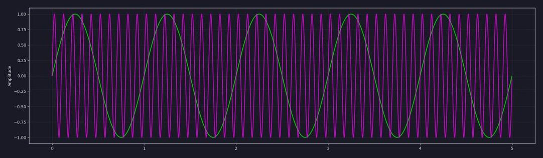
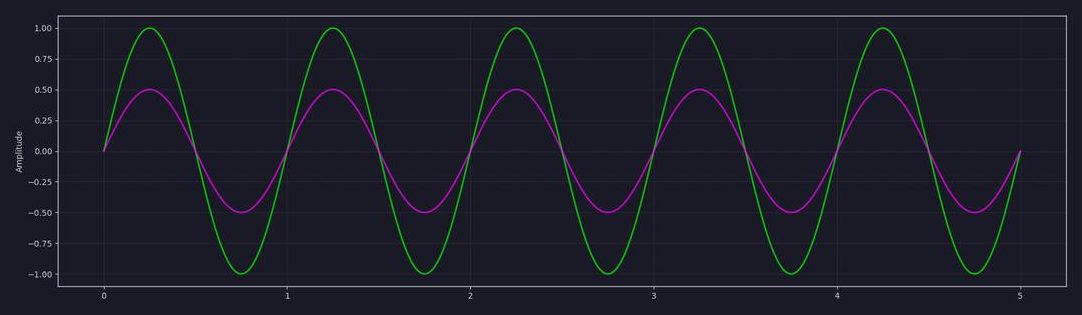
- AM (Amplitude Modulation) — the amplitude of the carrier changes with the signal. Information lives in the "skin" of the waveform, the envelope.
- FM (Frequency Modulation) — amplitude is held constant and the frequency is varied instead. The waveform bunches up and spreads out to carry the message.
- PWM (Pulse Width Modulation) — a fundamentally different approach. The voltage is either fully on or fully off, and information is expressed by the width of the pulse. It is the scheme most at home in a world of ones and zeros.
Modulation as a concept was formalised in 1920s radio engineering. Carson's 1922 paper "Notes on the Theory of Modulation" was the first clear statement of which frequency components appear, and over how wide a band, when information is placed on a carrier. The "Carson bandwidth rule" still used a century later to estimate FM bandwidth comes from that work. A directional speaker simply substitutes ultrasound for radio waves as the carrier; it inherits the grammar wholesale.
Before comparing the three, one distinction is worth fixing in advance. AM and FM are rules that decide which physical quantity the information is inscribed onto. PWM is closer to a rule about how that waveform is driven out with power. Lined up side by side the three look like equal competitors, but in an actual design they sit at different layers. The conclusion of this article converges on exactly that point.
AM — the envelope as a vessel
The AM equation and its sideband structure were established back in Part 2: swing the carrier amplitude in proportion to the signal and sidebands appear either side of the carrier frequency, so that audio up to 20kHz placed on a 40kHz carrier occupies 20~60kHz. Here we move to the next question — how is the transmitted power divided across that band?
Accounting for the power split reveals AM's character. For a single sine tone at modulation index m, the fraction of total average power carried by the sidebands is m² / (2 + m²). The carrier component itself contains no information at all, yet it takes everything that is left. The numbers work out as follows.
| Modulation index m | Carrier power share | Both sidebands | One sideband |
|---|---|---|---|
| 0.1 | 99.50% | 0.50% | 0.25% |
| 0.3 | 95.69% | 4.31% | 2.15% |
| 0.5 | 88.89% | 11.11% | 5.56% |
| 0.7 | 80.32% | 19.68% | 9.84% |
| 1.0 | 66.67% | 33.33% | 16.67% |
Every value in the table falls straight out of the single expression m² / (2 + m²). Even at m = 1.0, filled right up to the edge of over-modulation, the informative share is one third of the total; run politely at m = 0.3 and it drops to about 4%. For ordinary broadcasting the story would end with a complaint about wasted power. In a directional speaker the verdict flips. As we will see below, the air can only recover sound if the carrier is present alongside the sidebands. The carrier power that looks like waste is in fact the fuel that runs the demodulator.
AM's other virtue is simplicity. Encoding is a single multiplication, and the receiving end only has to follow the envelope. That is why a diode and a capacitor sufficed as an "envelope detector" in the radio era — and why, a century later, air itself can take over the job.
FM — noise immunity bought with bandwidth
FM never touches amplitude. As the signal rises the instantaneous frequency moves up, as it falls the frequency moves down, but the height of the waveform is identical from beginning to end. This property gives FM its famous advantage — natural noise rides mostly on amplitude, so a receiver can discard amplitude information entirely (with a limiter) and the message survives intact. Armstrong's 1936 paper demonstrated exactly this noise-suppression effect, and it is why music broadcasting migrated to FM.
The price is bandwidth. Carson's rule puts the practical occupied bandwidth of an FM signal at BW ≈ 2 × (Δf + f_m), where Δf is the frequency deviation (how far the carrier is pushed at peak signal) and f_m is the highest audio frequency. Sweeping the deviation ratio β = Δf / f_m gives the following.
| Scheme | Condition | Occupied bandwidth | Relative to 40kHz carrier |
|---|---|---|---|
| AM · SSB | audio 8kHz | 8kHz | 0.20x |
| AM · SSB | audio 20kHz | 20kHz | 0.50x |
| AM · DSB | audio 8kHz | 16kHz (32~48kHz) | 0.40x |
| AM · DSB | audio 20kHz | 40kHz (20~60kHz) | 1.00x |
| FM (β = 1) | audio 8kHz, Δf 8kHz | 32kHz | 0.80x |
| FM (β = 1) | audio 20kHz, Δf 20kHz | 80kHz | 2.00x |
| FM (β = 5) | audio 20kHz, Δf 100kHz | 240kHz | 6.00x |
The values come from substituting directly into 2·f_m for DSB, f_m for SSB, and Carson's 2(Δf + f_m) for FM. FM's attraction, its noise immunity, improves as β grows — but a "high fidelity" FM at β = 5 placed on a 40kHz carrier demands 240kHz of bandwidth, six times the carrier itself. A modulation that requires more bandwidth than its own carrier is not physically realisable; the spectrum would have to fold back through zero hertz. FM broadcasting's use of an 88~108MHz carrier is not an accident but the consequence of climbing to a place where the bandwidth can be afforded.
This table gives the directional-speaker designer their first piece of practical intuition. Within a 40kHz carrier budget the only usable options are the AM family, and even then with the audio band restricted. Why commercial directional speakers abandon the top octave and concentrate on the speech band is taken up directly in Part 14.
PWM — the language of power, not of information
PWM has a different texture from the other two. The output takes only two values, fully on and fully off, and the information lives in the fraction of each period spent switched on: the duty cycle. The key point comes next — pass that square wave through a low-pass filter and what remains is an average proportional to the duty cycle. Fifty percent duty gives half the supply voltage, seventy-five percent gives three quarters. In other words, PWM is a way of imitating an analogue amplitude using nothing but a switch.
Seen this way, PWM is not a competitor of AM and FM at the same layer. Transcribe the instantaneous amplitude of an AM signal into a duty cycle and you have a PWM signal; pass it through a filter — or through the transducer's own resonance — and the original AM waveform reappears. The information is still carried by AM; PWM is the vehicle that delivers it.
The reason to bother with PWM at all is one thing: efficiency. Heat in an amplifying device comes fundamentally from having voltage across the device and current through it at the same instant. A linear amplifier maintains that state continuously. A switching amplifier stays either fully on (nearly zero voltage) or fully off (zero current), so its losses are small in principle. The theoretical efficiency limits line up as follows.
| Amplifier class | Theoretical maximum | Basis | Efficiency in real use |
|---|---|---|---|
| Class A (series-fed) | 25% | peak load power ÷ constant DC draw | under 10% (worse as signal shrinks) |
| Class A (transformer-coupled) | 50% | same calculation, DC loss removed | around 20% |
| Class B/AB (push-pull) | 78.5% | π/4 | 39% at half of peak amplitude |
| Class D (switching) | above 95% | conduction loss only: R/(R + 2·R_ds) | 97.6% for 8Ω load and 0.1Ω R_ds |
Class B's 78.5% is the classical result of integrating a half sine and arriving at π/4; in practice the efficiency falls in proportion to amplitude, so half-scale drive gives 39% (see table). For music, whose average level sits far below its peaks, the effective efficiency of a linear amplifier is lower still. Class D loss, by contrast, is dominated by the on-resistance of the switch, so with 0.1Ω on-resistance into an 8Ω load the figure is 8 / (8 + 0.2) = 97.6%. Add switching loss and dead-time and the realistic number lands in the low-to-mid nineties.
PWM has its own price. A square wave produces a comb-shaped spectrum with strong components at every integer multiple of the switching frequency, spraying energy into bands you did not ask for. And how finely the duty cycle can be divided is the effective resolution, so the Nyquist argument of Part 11 returns here. To reproduce a 60kHz upper sideband the switching frequency must be at least 120kHz, and 300~600kHz in practice; adding a 10-bit duty resolution (quantisation SNR about 62dB) then requires a timer clock of 400kHz × 1024 ≈ 410MHz. That is beyond a cheap microcontroller, and it is why the drive stage of a directional speaker calls for dedicated logic or a high-speed timer peripheral.
AM vs FM — the trade-off radio already taught us
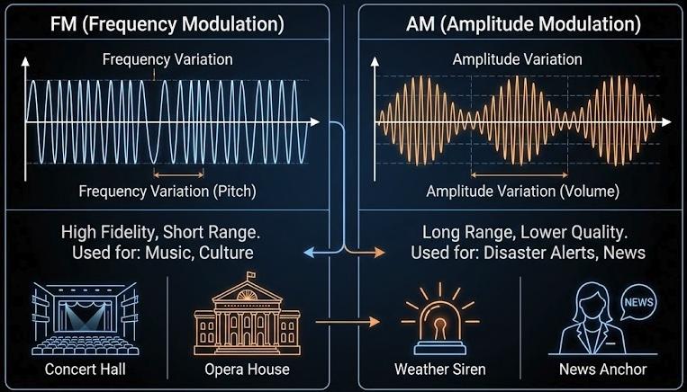
The difference in character between the two schemes has already been proven in radio broadcasting.
- FM — high fidelity, short reach: robust against noise (which mostly rides on amplitude), hence good sound quality. That is why music stations are on FM.
- AM — long reach, lower quality: poorer sound but it travels far. That is why emergency alerts and news use AM.
Reading that contrast as "one modulation scheme is superior" would be a mistake. FM broadcasts do not travel far because of the modulation but because FM stations use a high carrier frequency that propagates in straight lines and does not diffract past the horizon. AM travels far not through any merit of the modulation but because medium waves reflect off the ionosphere. The radio rule of thumb is therefore a joint result of "modulation scheme plus carrier band". On a stage where the carrier is pinned at 40kHz, that rule of thumb cannot simply be carried over; the question has to be re-derived from scratch.
The three schemes at a glance
Everything so far condenses into a single sheet. This table is the backbone of this instalment.
| Property | AM | FM | PWM |
|---|---|---|---|
| Handle carrying information | amplitude (envelope) | instantaneous frequency | pulse width (duty) |
| State of the envelope | varies with the signal | always constant | post-filter average follows the signal |
| Occupied band (20kHz audio) | 40kHz DSB / 20kHz SSB | 80~240kHz | comb at multiples of the switching rate |
| Immunity to amplitude noise | weak | strong | moderate (digital decision helps) |
| Matching amplifier | linear (Class A/AB) | linear or switching | switching (Class D) |
| Amplification efficiency | 25~78.5% theoretical ceiling | 78.5% theoretical ceiling | above 90% |
| Implementation difficulty | low (one multiplication) | moderate (phase integration) | moderate (needs a fast timer) |
| Can air demodulate it? | yes | no | not applicable — it is a vehicle |
| Role in a directional speaker | information encoding | unsuitable | power delivery |
The special condition of a directional speaker — the receiver is air
A radio has an electronic receiver, so it can demodulate any scheme you like. But the receiver of a directional speaker is air. And as Berktay's law from Part 7 tells us, air returns as sound only the second time derivative of the square of the envelope. Air, in other words, is a fussy receiver that can decode nothing but information written into amplitude.
That one line decides the fate of the three candidates.
- FM is eliminated on principle. The envelope of an FM signal is a constant. Square a constant and it is still constant; differentiate a constant twice and you get exactly zero. No matter how powerful the FM ultrasound, the audible sound air produces is theoretically nil. FM's one strength, noise immunity, is meaningless here — demodulation never happens in the first place.
- AM passes. The envelope is the information, and what air does is envelope detection, so the two are matched. The "square" and "double derivative" habits of air do bring distortion and a lack of bass if left uncorrected, and correcting them is the subject of Parts 13 and 14.
- PWM is not on trial. It is not a signal handed to the air for decoding at all, but a way of pushing an AM waveform efficiently to the transducer.
The answer for a directional speaker is therefore not a choice among three but a two-stage arrangement: encode with AM, drive with PWM. Part 13 assembles that arrangement against real circuits and real transducer characteristics.
Three common misconceptions
Misconception 1 — "FM sounds better, so a directional speaker should use FM." FM's quality advantage assumes an electronic receiver equipped with a limiter and a discriminator. Air has no such circuitry. Since the demodulator cannot be changed, the signal must be shaped to fit it.
Misconception 2 — "PWM is a better modulation scheme than AM." They are at different layers. PWM expresses amplitude as time, so after low-pass filtering it becomes amplitude information again. It does not replace AM; it carries AM.
Misconception 3 — "Carrier power is waste because it holds no information." True in communications, which is precisely why SSB and suppressed-carrier schemes were developed. In a directional speaker, however, the carrier is the reference signal that lets the air-as-demodulator work at all. Remove it and the reference for demodulation disappears, leaving badly distorted sound. It is the classic case of a communications truism failing to transfer.
Summary
Modulation loads information onto the amplitude (AM), frequency (FM) or pulse width (PWM) of a carrier. AM is narrow-band, simple to implement, and leaves information in the envelope; FM is robust against noise but demands a bandwidth a 40kHz carrier cannot supply; PWM is less a way of carrying information than a way of delivering power at over 90% efficiency.
In ordinary communications you choose by application. But the demodulator of a directional speaker is not a circuit — it is non-linear air. Air reads only the envelope, so FM is silent on principle, and the answer narrows to encode with AM, drive with PWM. The next instalment places that conclusion on top of a real constraint, the narrow resonant band of the transducer, and compares distortion-suppressing modulation schemes quantitatively.
About this series
"The Science of Directional Speakers" runs in the following order.
- What is a directional speaker — the flashlight of sound
- Loading sound onto inaudible sound — first steps in operating principle
- Applications of directional speakers — exhibition, safety, retail, office
- What is ultrasound — definition, types, propagation
- Why ultrasound — generation principles and application map
- The magic of air becoming a speaker — PAA non-linear acoustics
- PAA theory in depth — Berktay, Westervelt, KZK
- Aiming sound — phased arrays and beamforming
- The piezoelectric effect — the moment electricity becomes sound
- Ultrasonic transducer design — resonance and arrangement
- The Nyquist theorem — the starting point of digital sound
- Introduction to modulation — AM, FM and PWM at a glance (this instalment)
- Coming next: modulation strategy for directional speakers, signal processing optimisation
This series is a blog adaptation of self-produced lecture material researched and compiled on ultrasonic directional audio technology. The figures are excerpted from that material.
References
- J. R. Carson, "Notes on the Theory of Modulation," Proc. IRE 10(1), 57 (1922) : the first formal treatment of the sidebands and occupied bandwidth created by modulation; source of BW ≈ 2(Δf + f_m) used in the FM bandwidth table
- E. H. Armstrong, "A Method of Reducing Disturbances in Radio Signaling by a System of Frequency Modulation," Proc. IRE 24(5), 689 (1936) : the original demonstration of FM's noise-suppression effect, basis for the claim that FM resists amplitude noise
- H. O. Berktay, "Possible exploitation of non-linear acoustics in underwater transmitting applications," JSV 2(4), 435 (1965) : the relation stating that recovered sound is the second derivative of the squared envelope; the mathematical basis for eliminating FM
- P. J. Westervelt, "Parametric Acoustic Array," JASA 35(4), 535 (1963) : the theory that non-linear interaction of two ultrasonic components generates a difference frequency
- M. Yoneyama et al., "The audio spotlight: An application of nonlinear interaction of sound waves to a new type of loudspeaker design," JASA 73(5), 1532 (1983) : experimental recovery of audible sound from AM-modulated ultrasound using an airborne transducer array
- T. Kamakura et al., "Parametric loudspeaker — characteristics of acoustic field and suitable modulation of carrier ultrasound," Electron. Commun. Jpn. 74(9), 76 (1991) : comparison of how sound field and distortion vary with the carrier modulation scheme
- "Dynamic single sideband modulation for realizing parametric loudspeaker," AIP Conf. Proc. 1022, 613 (2008) : background for the SSB row of the bandwidth table; sideband processing that addresses bandwidth and distortion together
- US 5,889,870 — Acoustic heterodyne device and method : patent covering the recovery of audible sound from an audio-modulated ultrasonic carrier
- Amplitude modulation — Wikipedia : the basic AM relations including the sideband power fraction m²/(2+m²)
- Carson bandwidth rule — Wikipedia : the approximation used to compute the FM bandwidth table
- Pulse-width modulation — Wikipedia : duty cycle versus average voltage, and an overview of the comb spectrum
- Class-D amplifier — Wikipedia : loss structure and efficiency range of switching amplifiers; basis for the Class D row of the efficiency table