The Science of Directional Speakers #13 — The Directional Speaker's Modulation Strategy: Resonance and PWM

Part 12 set up a contest, and this is the verdict. AM, FM and PWM each step into the ring of the directional loudspeaker, and each receives a ruling from two judges at once — the theory (Berktay) and the hardware (transducer resonance). The short version: the winner is a two-stage strategy, "design in AM, drive with PWM."

FM is eliminated — a verdict handed down by mathematics

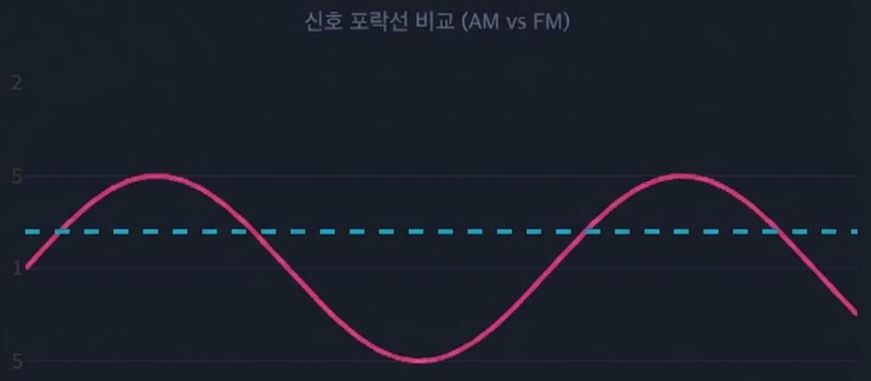
Recall Berktay's law from Part 7 — the sound the air restores is P_aud(t) ∝ ∂²/∂t² [E(t)]², the square of the envelope E(t) differentiated twice. But the amplitude of an FM signal is constant. Differentiate a constant and you always get zero — in theory an FM signal can produce no sound at all in air.

And yet, if you radiate FM in a lab, you do hear something. Why? Not because the air demodulated it, but because the transducer forcibly converted FM into AM (slope detection). When the frequency wanders across the steep flank of a narrow resonance curve, the output amplitude wanders with it, and unintended AM appears. The price is steep: the resonance flank is not linear, so severe harmonic distortion appears, and energy that falls outside the resonance is dissipated as heat, which can destroy the element. FM is eliminated.

Eliminated, however, does not mean abandoned by researchers. Because its amplitude is constant, FM lets an amplifier run deep in saturation, which is excellent for power efficiency, and attempts to exploit that advantage have continued — typically by modelling the nonlinear transfer of the resonance curve and pre-inserting its inverse into the signal (Hatano and colleagues, 2017). Using FM therefore means treating the transducer, not the air, as the demodulator, and modelling that demodulator's nonlinearity in full. Given that the resonance curve drifts with part spread and temperature, the same effort spent on AM pre-processing pays back far more.

What the hardware demands — reading the resonance curve

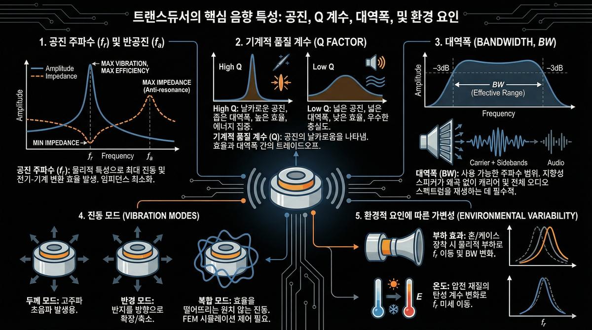
Why is the transducer's response so narrow-minded? This is where Parts 9 and 10 rejoin the story. A transducer delivers maximum displacement and maximum efficiency at its resonance frequency f_r (impedance minimum); the sharpness of that curve is set by the quality factor Q, and the usable width by the bandwidth BW. For a directional loudspeaker to reproduce without distortion, the carrier and the entire sideband structure must fit inside that bandwidth. Add that f_r shifts slightly with temperature or with a horn attached, and the stage turns out to have very little room.

This constraint only becomes real in numbers. By the definition of a resonant system, BW = f_r / Q, and double-sideband modulation occupies twice the audio ceiling, so the audio ceiling you can carry is BW / 2. Computed for a 40kHz carrier, the picture looks like this.

Transducer Q	-3dB bandwidth (f_r = 40kHz)	Audio ceiling, DSB	Audio ceiling, SSB	Practical meaning
3	13.3kHz	6.7kHz	13.3kHz	Wide, but sensitivity and output are badly hurt
5	8.0kHz	4.0kHz	8.0kHz	Ample for voice announcement, muffled for music
10	4.0kHz	2.0kHz	4.0kHz	Around the floor for speech intelligibility
20	2.0kHz	1.0kHz	2.0kHz	Typical of high-sensitivity elements; even speech is tight
30	1.33kHz	0.67kHz	1.33kHz	Alarm tones and single tones only

The table makes the trade explicit. Raise Q and you buy output with bandwidth. The reason a piezoelectric element is operated at resonance is to obtain far greater displacement from the same voltage, and that gain is bought precisely by selling bandwidth. This is why directional loudspeaker design feels uniquely cramped: a parametric array builds sound in proportion to the square of the ultrasonic pressure, so output cannot be surrendered, yet surrendering bandwidth leaves no audio to reproduce.

Real arrays therefore either mix elements whose f_r values differ slightly so that the composite response is wider, or deliberately lower the mechanical Q with a rear air cavity and matching layers. Neither is free; each is a trade in which a little of the right-hand column is bought with the left.

Where the symmetry of resonance comes from

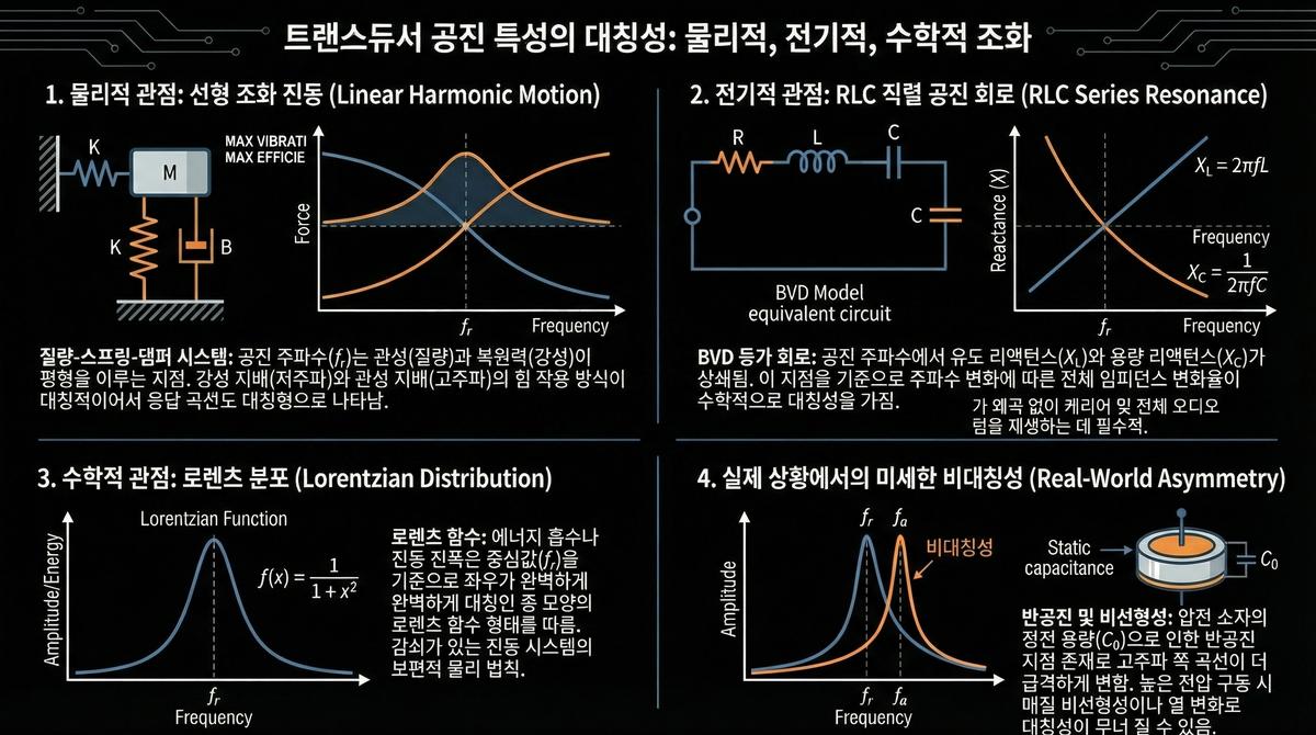
One property deserves attention — the resonance curve is symmetric about f_r. Physically it is a mass-spring-damper oscillator; electrically it is a series RLC resonance (the BVD equivalent circuit); mathematically it is a Lorentzian. All three views draw the same bell-shaped, symmetric curve. That symmetry will decide the next choice.

The convergence of those three views is no coincidence. That a piezoelectric vibrator reduces, as a circuit, to one series RLC branch plus a parallel static capacitance was already established in 1928 (Van Dyke). Mechanical mass maps to inductance, stiffness to capacitance, and frictional loss to resistance. Near resonance the response of a lightly damped second-order system is identical on both sides of f_r. In short, the transducer can barely distinguish a component 1kHz below f_r from one 1kHz above it. That inability decides the conclusion of the next section in advance.

The two faces of AM — DSB or SSB

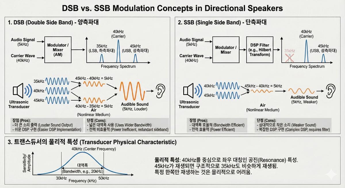
The surviving AM branch itself forks. Put 5kHz of speech onto a 40kHz carrier and you create 35kHz (lower sideband) and 45kHz (upper sideband). Do you radiate both (DSB) or just one (SSB)?

• DSB (double sideband) — both sidebands interact with the carrier, so the sound is louder, and the DSP is easy to implement. In exchange it occupies wide bandwidth and uses power inefficiently.
• SSB (single sideband) — bandwidth and power efficiency are good, but the sound is weaker and it demands elaborate DSP filtering such as the Hilbert transform.

Here the symmetry intervenes. Because the resonance is symmetric about 40kHz, if 45kHz is radiated then 35kHz is structurally radiated at nearly the same level. Emitting only one sideband is physically difficult, which is why practical designs generally start from a DSB baseline.

Beyond symmetry, SSB has one more property worth spelling out. What the air reads is not a spectrum but an envelope, and keeping only the upper sideband makes the envelope a blend of the original signal s and its Hilbert transform ŝ. Squaring it gives 1 + m·s + (m²/4)(s² + ŝ²), and the last bracket is interesting: for a single sine tone, s² + ŝ² is identically one — a constant — so it disappears the moment you differentiate. In other words, the intrinsic distortion of SSB for a single tone is exactly zero.

The problem is that real speech and music are not single tones. With two or more tones s² + ŝ² is no longer constant, and components that were never in the source survive near the difference frequency. The bandwidth halved, but the distortion did not vanish entirely. That is the backdrop for recursive SSB schemes, which whittle the residual down by iteration, and for weighted DSB schemes, which give the two sidebands unequal weights.

The scorecard

Here is the whole discussion on one page. Occupied bandwidth is expressed with the audio ceiling written as f_a, and "intrinsic distortion" is the share that follows from the equations regardless of component quality.

Scheme	Envelope E(t)	Occupied bandwidth	Intrinsic distortion	Computation	Fit to the resonance	Verdict
DSB-AM (uncorrected)	1 + m·s(t)	2 f_a	Second harmonic = m for a single tone (50% at m = 0.5)	One multiply	Natural fit to a symmetric curve	Baseline
Square-root AM (DSB)	√(1 + m·s(t))	2 f_a to 8 f_a, set by m	Cancels in theory; residual equals what was truncated	Square root plus band limiting	Overruns the band when m is large	Practical standard
SSB	Signal blended with its Hilbert transform	f_a	Zero for one tone, residual for many	Hilbert transform	Symmetry revives the other side	Partially adopted
Recursive SSB / weighted DSB	Iteratively corrected envelope	f_a to 2 f_a	Falls with iteration count	Iteration and latency	Good	Advanced option
FM	Constant	Narrow	Zero self-demodulated output; relies on slope detection	Low	Entirely at the mercy of the flank	Eliminated
Square-wave PWM drive	Duty cycle	Fundamental plus odd harmonics	Switching harmonics, outside the band	One comparator	Resonance acts as the reconstruction filter	The answer for the power stage

The second row connects to the conclusion of the whole series. The relation seen in Part 7 — "restored sound ∝ second derivative of the squared envelope" — prescribes its own cure: put a square root on the envelope in advance and it cancels the square exactly. The catch is that the square-root operation manufactures harmonics that were not in the signal, widening the envelope's own bandwidth, and that widened bandwidth runs straight into the wall of transducer Q. How far to push the square root and where to truncate it is the subject of Part 14.

Distortion suppression in numbers

Let us turn the "intrinsic distortion" column into actual figures. For each scheme the envelope E(t) was constructed directly, squared and differentiated twice as Berktay's relation prescribes, and the recovered audio was analysed for components that were not present in the source. Conditions: modulation index m = 0.7, all schemes normalised to the same peak drive voltage, and two test signals — a single tone (1kHz) and two tones (1.0kHz + 1.3kHz). The two-tone case is included because, as the previous section explained, a single tone does not expose SSB's weakness.

Scheme	Single-tone distortion	Two-tone distortion	Recovered output	Envelope bandwidth	Implementation
DSB-AM (uncorrected)	57.4%	50.6%	0 dB (reference)	2 f_a	one multiplication
Square-root AM (unlimited)	0%	0%	−1.4 dB	3 f_a (−40dB) to 5 f_a (−60dB)	one square root
Square-root AM (limited to 3.2kHz)	8.0%	12.8%	−1.3 dB	about 2.5 f_a	square root plus low-pass
SSB (carrier plus upper sideband)	0%	0.80%	−2.0 dB	f_a	Hilbert transform
Recursive SSB / weighted DSB	falls with iteration	falls with iteration	similar to SSB	f_a to 2 f_a	iteration plus latency
Square-wave PWM drive	no envelope distortion	switching 3rd at −38dB	+4.2 dB	fundamental plus odd harmonics	one comparator

What the table shows is not a ranking but a set of exchange rates. The 57% distortion of uncorrected DSB matches exactly the relation m / √(1 + m²) from Part 7 evaluated at m = 0.7, and applying the square root drives that distortion numerically to zero. In exchange the envelope bandwidth stretches to three or four times f_a — up to eight times as m approaches one — and the moment that band is forcibly cut at 3.2kHz the distortion returns at 8~13%. Square-root correction is realised only to the extent that the transducer grants bandwidth.

The SSB row is attractive: half the bandwidth for under one percent distortion. But if the suppressed sideband is revived by the symmetric resonance, that 0.80% will not hold. The last row is different in kind — what square-wave PWM produces is not envelope distortion but switching harmonics, and as the next two sections show, the resonance curve filters those out by itself. At the same supply voltage the fundamental grows by 4/π, lifting the ultrasonic pressure by 2.1dB; because the recovered audio scales with the square of that pressure, the gain becomes +4.2dB.

PWM — the language of power

The remaining question is how to amplify this AM signal efficiently. A linear amplifier (Class A/AB) that raises amplitude continuously is like a tap held half open, throwing the surplus away as heat (below 70% efficiency). PWM with a switching amplifier (Class D) turns the tap fully on and fully off and regulates the flow by how long it stays open — above 90% efficiency, minimal loss. When hundreds of transducers have to be driven, efficiency is not a preference but a condition of survival.

"Below 70%" has an arithmetic basis. The theoretical maximum efficiency of a push-pull linear stage (Class B) is π/4 ≈ 78.5%, reached only when the output swing fills the supply rail, and real circuits fall short of that because of bias current and headroom. In a switching stage, by contrast, loss arises only in the conduction resistance and during switching transitions.

The gap widens dramatically in this application because the carrier is always on. In ordinary audio the average level sits far below the peak, so even a linear amplifier draws little on average. A directional loudspeaker, however, emits its 40kHz carrier near full output whether the programme is loud or quiet. Under linear amplification that permanent load becomes permanent heat, and in a panel carrying dozens or hundreds of elements that heat returns as f_r drift and shortened life.

Why hitting it with a square wave is allowed

Once linear amplification is abandoned, what reaches the transducer is not a smooth sinusoid but a hard-edged square wave. In an audio amplifier that would be alarming; here it is an advantage, for two reasons.

First, the square wave's fundamental is larger. Expand a unit-amplitude square wave as a Fourier series and the fundamental has amplitude 4/π ≈ 1.27, about 2.1dB above a sinusoid of the same amplitude. That means stronger ultrasound from the same supply rail, and since a parametric array builds sound from the square of the ultrasonic pressure, those 2.1dB return as close to a doubling in the restored audio.

Second, the unwanted harmonics are discarded by the resonance itself. A square wave carries only odd harmonics, with amplitudes falling as 1/n. For a 40kHz square wave the third harmonic sits at 120kHz, 9.5dB below the fundamental, and the fifth at 200kHz, 14dB below. As the earlier table showed, a Q = 10 transducer has a -3dB span of merely 40kHz ± 2kHz. At 120kHz the element is so far outside that span that it barely responds at all. The narrow bandwidth that was the villain now works as a free low-pass filter.

Square-wave drive, then, is not a crude shortcut but a design that repurposes a physical property of the element as a filter. It is not free either: harmonic energy pushed outside the resonance never becomes sound, and ends as heat inside the element or as electromagnetic noise on the wiring. That is why gate control that softens the switching edges, and shielded harnesses, are never absent from a real build.

The drive pipeline — assembled in three stages

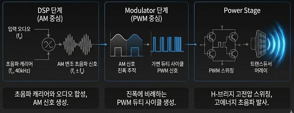
The real drive chain therefore assembles like this. ① The DSP stage synthesises the audio onto the 40kHz carrier and designs the AM signal — building the waveform shell that the air will decode. ② The modulator stage substitutes PWM duty cycle for the amplitude information. ③ The power stage has an H-bridge switch the high voltage and launch high-energy ultrasound.

Each stage speaks a different language: ① handles numbers, ② lengths of time, ③ quantities of charge. Something is lost at every boundary, so the error budget must be split three ways — in ① an inadequate sampling rate folds the sidebands back into the band, in ② insufficient duty resolution parks quantisation noise beside the carrier, in ③ excessive dead time distorts the duty ratio. The sampling theorem of Part 11 is a stage-① problem, and the modulation index of Part 14 straddles ① and ②.

Three common misconceptions

• "FM's constant amplitude is an advantage here." The opposite. Constant amplitude means the envelope carries no information, and the envelope is all the air reads. The amplification-efficiency benefit is already delivered, in larger measure, by PWM.
• "SSB halves the bandwidth, so it solves the transducer problem." Only half true. The occupied bandwidth shrinks, but the symmetric resonance revives the opposite sideband, and with more than one tone present the surviving envelope no longer matches the source, so fresh distortion appears.
• "Class D sounds poor, so high-end units use linear amplification." This transplants a general-audio prejudice. What sets final quality here is not the amplifier's waveform fidelity but the accuracy of the envelope, and square-wave harmonics are filtered out by the transducer's own resonance.

Summary

Because the air listens only to the envelope, FM is silent in principle — and when it is audible, that audibility comes bundled with distortion and heat. Information is therefore encoded in AM. Because the resonance is symmetric, practice centres on DSB, and power is solved with PWM switching. That same narrow resonance is both the chief obstacle and a free filter that removes square-wave harmonics. Only the last piece of the series remains — how far to apply square-root pre-compensation and where to set the modulation index, which is to say the signal processing that optimises the whole chain.

Series guide

"The Science of Directional Loudspeakers" runs in the following order.

1. What is a directional loudspeaker — a flashlight for sound
2. Putting sound on an inaudible sound — first steps in the operating principle
3. Applications — exhibition, safety, retail, office
4. What is ultrasound — definition, types, propagation
5. Why ultrasound — generation principles and a map of applications
6. The magic of air becoming a loudspeaker — PAA and nonlinear acoustics
7. PAA theory in depth — Berktay, Westervelt, KZK
8. Aiming sound — phased arrays and beamforming
9. The piezoelectric effect — the moment electricity becomes sound
10. Ultrasonic transducer design — resonance and layout
11. The Nyquist theorem — the starting point of digital sound
12. Introduction to modulation — AM, FM and PWM at a glance
13. Modulation strategy for directional loudspeakers — resonance and PWM (this part)
14. Next: signal processing optimisation — bandwidth and modulation index (finale)

This series reworks self-produced lecture material on ultrasonic directional audio, researched and compiled by the author, into blog form. The figures are drawn from that material.

References

• H. O. Berktay, "Possible exploitation of non-linear acoustics in underwater transmitting applications," JSV 2(4), 435 (1965) : source of the relation P_aud ∝ ∂²/∂t²[E(t)]² and the basis for eliminating FM
• H. O. Berktay, D. J. Leahy, "Farfield performance of parametric transmitters," JASA 55(3), 539 (1974) : the far-field validity range and limiting conditions of the envelope approximation
• T. Kamakura et al., "Parametric loudspeaker — characteristics of acoustic field and suitable modulation of carrier ultrasound," Electron. Commun. Jpn. 74(9), 76 (1991) : acoustic field and distortion compared across carrier modulation schemes
• "Dynamic single sideband modulation for realizing parametric loudspeaker," AIP Conf. Proc. 1022, 613 (2008) : SSB-family modulation addressing bandwidth and distortion together
• Y. Wang et al., "SSB modulation of the ultrasonic carrier for a parametric loudspeaker," Int. Conf. Electronic Computer Technology, 669 (2009) : implementation of single-sideband modulation and its residual distortion
• P. Ji, W.-S. Gan, E.-L. Tan, J. Yang, "Performance analysis on recursive single-sideband amplitude modulation for parametric loudspeakers," IEEE ICME, 748 (2010) : reducing SSB residual distortion by iteration
• Y. Hatano, C. Shi, Y. Kajikawa, "Compensation for nonlinear distortion of the frequency modulation-based parametric array loudspeaker," IEEE/ACM TASLP 25(8), 1709 (2017) : modelling and compensating transducer nonlinearity under FM drive
• K. S. Van Dyke, "The piezo-electric resonator and its equivalent network," Proc. IRE 16(6), 742 (1928) : origin of the BVD equivalent circuit and of the symmetry of the resonance curve
• A. R. Oliva, S. S. Ang, T. V. Vo, "A multi-loop voltage feedback filterless class-D switching audio amplifier using unipolar pulse-width-modulation," IEEE Trans. Consumer Electronics 50(1), 312 (2004) : structure and loss mechanisms of a PWM switching output stage
• US 5,889,870 — Acoustic heterodyne device and method : patent on obtaining audible sound from an ultrasonic carrier
• Class-D amplifier — Wikipedia : overview of switching amplification and its efficiency