The Science of Directional Speakers #14 — Signal Processing Optimization: Bandwidth and Modulation Index

This is the final instalment of the series. Every component is assembled — what remains is the signal-processing finishing work that lifts the system to commercial product quality. Two keywords: pre-processing and modulation index.

The carrier is not a component, it is software

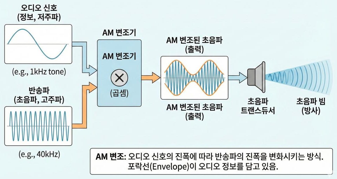
Let us correct an easy misconception first. The carrier and the modulated wave of a directional loudspeaker are not produced by a physical part humming away; they are generated mathematically by a software algorithm inside a DSP or MCU. AM modulation is really one line of multiplication — audio signal times 40kHz carrier. The envelope of the result holds the audio information, and all of this arithmetic runs on top of the 192kHz sampling we saw in Part 11.

That fact has a practical consequence: sound quality can change with a firmware update alone, without touching the transducer or the amplifier. The choice of modulation scheme from Part 13, and the pre-processing filters and modulation-index management in this instalment, all live in code. Put the other way round, software cannot exceed the limits the hardware has already set. Half of this instalment is the work of confirming, in numbers, exactly where those limit lines are drawn.

Stage-by-stage processing — pre-processing is half the job

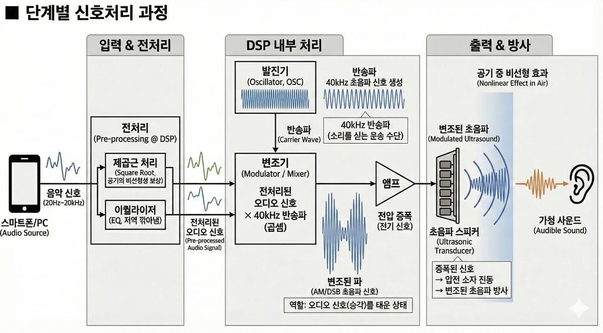
Follow the signal path of a real product and the part that decides quality is the pre-processing that happens before modulation.

1. Square root — remember Berktay's law from Part 7? Air returns the square of the envelope as sound. So if you apply a square root to the signal in advance, it cancels against the air's squaring and the original is restored. Pre-compensating the distortion of a nonlinear demodulator with mathematics is the single most elegant move in this system.
2. Equaliser — cutting the bass away — because of the transducer bandwidth limit from Part 13, low-frequency components far from the carrier cannot be carried properly anyway and leave only distortion. Removing unreproducible bass in advance cuts both distortion and wasted energy.
3. Inside the DSP, then out — an oscillator makes the 40kHz carrier, the modulator multiplies it with the pre-processed audio, an amplifier raises the voltage and the transducer array radiates. The air takes care of the rest.

The second item may sound strange. You would expect the effort to go into rescuing the bass, not cutting it away. Let us face that reason head-on.

The bass wall — what it costs to undo 12dB per octave

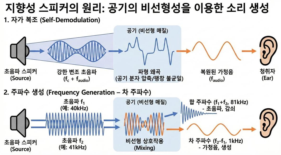
Berktay's relation says the recovered sound is the second derivative of the squared envelope. One differentiation means a weight proportional to frequency, so two differentiations multiply by frequency squared. An amplitude proportional to the square of frequency is, in decibels, a slope of 12dB per octave. A parametric loudspeaker therefore loses 12dB of bass with every octave by construction. That is the root cause of the thin, sharp timbre of the "flashlight of sound" from Part 1.

Could we not simply push the bass back up with an equaliser and flatten it? Working out the numbers shows immediately why not. Taking 5kHz as the reference point, here is how many decibels of boost each frequency needs to reach the same level.

Target frequency	Octaves below 5kHz	Boost required	Envelope amplitude ratio
4,000Hz	0.32	+3.9 dB	1.6x
2,000Hz	1.32	+15.9 dB	6.2x
1,000Hz	2.32	+27.9 dB	25x
500Hz	3.32	+39.9 dB	98x
200Hz	4.64	+55.7 dB	611x
100Hz	5.64	+67.7 dB	2,434x

The values come from the single expression 12 × log₂(5000 ÷ f), and the last column converts those decibels into a voltage ratio. What makes this decisive is that the envelope amplitude has a ceiling. The modulation index m cannot exceed one, so the headroom available to the envelope is at best a factor of a few — yet flattening 1kHz demands 25 times, and 100Hz demands 2,434 times. Pushing the EQ to rescue 100Hz would shove every other band 68dB below it.

The practical choice is therefore not "make it flat" but "decide where to give up". Typically everything below 200~300Hz is cut outright, and only an octave or two above that is partially corrected. If you do not cut it, that content never becomes sound and merely eats the envelope's headroom, which in the end reduces the loudness of the bands you can actually hear. That is why a bass-cutting EQ is not a measure that "throws the bass away" but one that recovers loudness in the mid and high band. Research into psychoacoustically reinforcing low-frequency perception, or into equalising sub-arrays separately to shape the response, continues precisely because this wall is physically so solid.

The decision to cut bandwidth — why the speech band

There is a wall at the top end too. As Part 13 showed, the usable width of a transducer is BW = f_r / Q, and double-sideband modulation consumes twice the audio ceiling. On a 40kHz carrier, the Q you can tolerate depends on where you place that ceiling.

Audio ceiling	Occupied spectrum	Bandwidth needed	Maximum allowable Q	Feasibility
20kHz (full audio)	20~60kHz	40kHz	1.00	effectively impossible
16kHz	24~56kHz	32kHz	1.25	close to impossible
8kHz (wideband speech)	32~48kHz	16kHz	2.50	possible with low-Q elements
4kHz (standard speech)	36~44kHz	8kHz	5.00	comfortable

Read alongside the Q table of Part 13, the picture completes itself. An element whose Q was raised to 20~30 for sensitivity has only 1.3~2kHz of bandwidth, which puts its audio ceiling below 1kHz. Conversely, carrying a full 20kHz of audio demands Q down at 1, and at that Q the sound pressure collapses and the parametric array stops working. The door that is actually open between those two walls is the speech band.

Fortunately speech tolerates band limiting well. The classic study of speech intelligibility showed that the information contributing to intelligibility is spread over a wide frequency range but concentrated heavily in the midband, and the telephone network has carried conversation on 300~3,400Hz for nearly a century as living proof. Directional loudspeakers found their first footing in announcements, exhibition commentary and warning tones not through marketing but because the band physics allowed happened to be the band of the human voice.

Modulation index m — how full to fill the vessel

The last handle is the modulation index, m. The definition is simple: the ratio of audio amplitude to carrier amplitude. Intuitively it measures how fully the "contents" of audio are packed into the "vessel" of ultrasound.

• Low m (say 0.1) — the ultrasound goes out strongly, but the audio swing inside it is tiny, so the demodulated sound is quiet.
• High m (say 1.0) — the carrier amplitude is exploited fully and the sound is loud and clear.

From this comes the loudness formula of a directional loudspeaker — perceived loudness = ultrasonic SPL + modulation index m. Because the demodulated audible pressure is proportional to the square of the ultrasonic pressure and to m, a transducer blasting 130dB of ultrasound will produce no sound at all if m is near zero. Filling m first, before raising output, is the correct order of operations.

Raising m, however, has a price — and the price is not only distortion but bandwidth. The square-root pre-processed envelope √(1 + m·s) manufactures harmonics that were never in the signal, and how many of those harmonics remain significant depends on m. With an audio ceiling of 4kHz and harmonics counted as significant down to −40dB, the numbers are these.

Modulation index m	Significant envelope harmonics	DSB occupancy	Maximum allowable Q	Relative recovered level	THD if uncorrected
0.3	2nd	16kHz	2.50	−10.5 dB	28.7%
0.5	2nd	16kHz	2.50	−6.0 dB	44.7%
0.7	3rd	24kHz	1.67	−3.1 dB	57.3%
0.9	4th	32kHz	1.25	−0.9 dB	66.9%
1.0	8th	64kHz	0.62	0 dB (reference)	70.7%

Three calculations built this table. The harmonic order is obtained by expanding √(1 + m·cos θ) as a Fourier series and counting the highest order still above −40dB relative to the fundamental; the occupancy is that order × 4kHz × 2 for double sideband; the allowable Q is 40kHz ÷ occupancy. The last column is the relation m / √(1 + m²) from Part 7.

This table is the most important one in the instalment. Going from m = 0.5 to m = 1.0 buys 6dB of loudness but quadruples the required bandwidth, from 16kHz to 64kHz. Supporting that 64kHz would need Q at or below 0.62, and a transducer that soft cannot generate the ultrasonic pressure the array needs. In other words a design that fills m to the brim cannot exist, and practice lands around m = 0.5~0.7 — surrendering 6dB of loudness in order to buy bandwidth and low distortion together.

Optimising m — gain, normalisation, compression

You cannot simply crank m upward either. The moment m exceeds one, over-modulation crushes the waveform. The practical target is "exactly m = 1.0 at the peak", and the ladder has three rungs.

1. Input gain — adjust the audio level at the preamplifier or DSP input so that the signal peak just touches m = 1.0.
2. Normalisation — fixed gain alone leaves m too low on quiet material and tears on loud material. Firmware brings the running maximum of the input close to digital full scale in real time.
3. Compressor / limiter — hold down instantaneous peaks to prevent over-modulation while keeping the average m high. It is the same principle as loudness management in broadcast audio.

Why the third item matters so much is explained by crest factor, the ratio of peak to average. Align the peak with m = 1.0 and the average modulation index falls below it by exactly the crest factor, and the average level of the recovered sound falls the same amount.

Crest factor	Typical material	Average modulation index	Average recovered level
18 dB	uncompressed classical recording	0.126	−18.0 dB
12 dB	ordinary music track	0.251	−12.0 dB
9 dB	lightly treated narration	0.355	−9.0 dB
6 dB	speech compressed for broadcast	0.501	−6.0 dB
3 dB	heavily limited announcement	0.708	−3.0 dB

The average modulation index is ten raised to the power of (−crest factor ÷ 20). The message is unambiguous: on identical hardware, reducing the crest factor from 18dB to 6dB raises perceived loudness by 12dB. Twelve decibels obtained without a bigger amplifier and without more transducers, purely through signal processing. That is why a compressor in a directional loudspeaker is not "a compromise that hurts sound quality" but a core component. Over-compress, of course, and musical expression disappears, so the settings are split by use — heavy for announcements, light for background music.

The latency budget — the constraint of running in real time

All of the processing above has to finish the instant the input arrives. Budgeting how much time each stage consumes gives the following. Filter latency is computed as (taps − 1) ÷ 2 ÷ sample rate for linear-phase FIR.

Processing stage	Condition	Latency
Input A/D conversion	sigma-delta decimation filter	about 1.00 ms
Bass correction EQ	linear-phase FIR, 512 taps at 48kHz	5.31 ms
Block processing buffer	256 samples at 192kHz	1.33 ms
Hilbert transform (SSB family)	257 taps at 192kHz	0.67 ms
Band limiting after square root	129 taps at 192kHz	0.33 ms
PWM modulation and output stage	comparator and gate driver	0.05 ms
Total		8.70 ms

How should we read that 8.7ms? At a sound speed of 343m/s, 8.7ms is exactly the time sound takes to travel 3 metres. A listener 10 metres away waits 29.2ms for the air alone. The signal-processing latency of a directional loudspeaker is therefore equivalent to moving the speaker three metres further back, and in most installations it disappears into the propagation delay.

Two cases do demand a re-budget. One is an exhibit paired with video, where people notice a mismatch between picture and sound readily. The other is reinforcement in which the talker hears their own voice, where latency interferes with speaking. In both cases, converting the heaviest item — the bass correction EQ — from a linear-phase FIR to a minimum-phase IIR recovers most of that 5.31ms. It is a trade of phase behaviour for latency.

What this technology cannot do

Before closing the series, here are the limit lines that all these numbers draw, gathered in one place.

• It cannot deliver real bass. The 12dB/octave slope is not something a modulation scheme or a processing trick can remove; it comes out of Berktay's relation itself. The calculation that flattening 100Hz requires 2,434 times the amplitude is the height of that wall.
• It cannot carry full-band audio. Putting 20kHz of audio on a 40kHz carrier requires a transducer with Q at or below 1, and such an element cannot produce the sound pressure a parametric array needs.
• It cannot reach zero distortion. Square-root pre-processing cancels distortion exactly in theory, but the effect is realised only to the extent the transducer grants bandwidth. In Part 13's calculation, distortion returned at 8~13% the moment the band was cut.
• Loudness is expensive. Because the recovered sound scales with the square of the ultrasonic pressure, it looks as though 3dB more ultrasound buys 6dB more audio — but in practice element count and drive power rise together, and most of that power never becomes sound at all; it becomes heat.

This list is not an attempt to belittle the technology. Quite the opposite: it tells you precisely where the technology wins. Delivering speech-band information into a narrow angle with accuracy — that is what this technology does better than any other loudspeaker.

Closing the series — a journey of fourteen parts

"The Science of Directional Speakers" ends here. Looking back, it was a single sentence — load sound onto inaudible ultrasound (modulation and signal processing), aim it as a narrow beam (arrays and beamforming), and the air restores the sound by itself (the parametric array). Behind the "flashlight of sound" metaphor of Part 1 sits all of this physics, mathematics and engineering.

Retracing the question each instalment answered: Parts 1~3 asked what it is and what it is for; Parts 4~5 asked why ultrasound was chosen as the carrier; Parts 6~7 asked how air becomes a demodulator (Westervelt and Berktay); Part 8 asked how the beam is aimed; Parts 9~10 covered the material physics and resonance of the elements that make ultrasound; Part 11 gave the sampling rules for handling it digitally; Parts 12~13 laid out the grammar and the strategy of loading information; and this Part 14 covered how to tune all of it into a single signal chain.

One structure recurred throughout the journey: almost every gain was bought by selling something else. A narrow beam is purchased with low efficiency, high sound pressure with narrow bandwidth, loudness with wide spectral occupancy. Good design turned out to be knowing which side of each scale you can afford to give up for the job at hand. That is why the series drew so many tables — a decision can only be made when both pans of the scale carry real numbers.

Thank you for travelling this far. The series is complete, but new developments and experiments in the field will continue to appear on this blog.

Full series contents

1. What is a directional speaker — the flashlight of sound
2. Loading sound onto inaudible sound — first steps in operating principle
3. Applications of directional speakers — exhibition, safety, retail, office
4. What is ultrasound — definition, types, propagation
5. Why ultrasound — generation principles and application map
6. The magic of air becoming a speaker — PAA non-linear acoustics
7. PAA theory in depth — Berktay, Westervelt, KZK
8. Aiming sound — phased arrays and beamforming
9. The piezoelectric effect — the moment electricity becomes sound
10. Ultrasonic transducer design — resonance and arrangement
11. The Nyquist theorem — the starting point of digital sound
12. Introduction to modulation — AM, FM and PWM at a glance
13. Modulation strategy for directional speakers — resonance and PWM
14. Signal processing optimisation — bandwidth and modulation index (this instalment, final)

This series is a blog adaptation of self-produced lecture material researched and compiled on ultrasonic directional audio technology. The figures are excerpted from that material.

References

• H. O. Berktay, "Possible exploitation of non-linear acoustics in underwater transmitting applications," JSV 2(4), 435 (1965) : the relation stating that recovered sound is the second derivative of the squared envelope; basis for the 12dB/octave bass slope and for square-root pre-processing
• H. O. Berktay, D. J. Leahy, "Farfield performance of parametric transmitters," JASA 55(3), 539 (1974) : the farfield conditions under which the envelope approximation holds, and its limits
• M. Yoneyama et al., "The audio spotlight: An application of nonlinear interaction of sound waves to a new type of loudspeaker design," JASA 73(5), 1532 (1983) : the first airborne parametric loudspeaker experiment, including measured bass deficiency
• T. Kamakura et al., "Parametric loudspeaker — characteristics of acoustic field and suitable modulation of carrier ultrasound," Electron. Commun. Jpn. 74(9), 76 (1991) : sound field and distortion compared across carrier modulation schemes
• T. D. Kite, J. T. Post, M. F. Hamilton, "Parametric array in air: Distortion reduction by preprocessing," JASA 103(5), 2871 (1998) : the origin of the pre-processing approach to distortion reduction; basis for the square-root section
• P. Ji, W.-S. Gan, E.-L. Tan, J. Yang, "Performance analysis on recursive single-sideband amplitude modulation for parametric loudspeakers," IEEE ICME, 748 (2010) : distortion and bandwidth performance of pre-processing-based modulation
• F. Karnapi et al., "Method to enhance the low-frequency perception from a parametric array loudspeaker," JASA 110(5), 2741 (2001) : attempts to reinforce, perceptually, bass that is physically hard to reproduce
• C. Zhang et al., "Sub-array equalization technique for the parametric array loudspeaker to reduce nonlinear distortion," INTER-NOISE 263, 1497 (2021) : equalising sub-arrays separately to address response and distortion together
• J. Yang et al., "Preprocessing Methods of Parametric Array Loudspeakers," in Parametric Array Loudspeakers, 109 (2025) : a survey of pre-processing techniques including square root, SSB and iterative correction
• N. R. French, J. C. Steinberg, "Factors Governing the Intelligibility of Speech Sounds," JASA 19(1), 90 (1947) : the classic quantification of how each frequency band contributes to intelligibility; basis for the speech-band section
• H. E. Bass et al., "Atmospheric absorption of sound: Further developments," JASA 97(1), 680 (1995) : the basis for computing the energy a 40kHz carrier loses with distance
• US 5,889,870 — Acoustic heterodyne device and method : patent covering the recovery of audible sound from an audio-modulated ultrasonic carrier