TFT Device Parameters #02 — Transfer Curves: The Device's Résumé, Read by Gate Voltage

In the previous installment we read the output curve. Holding the gate voltage V_GS at a single value and sweeping the drain voltage V_DS, we watched the current rise straight, pass the knee and flatten out.

The output curve tells us how much the device can pass. But there are things it does not reveal directly: at which gate voltage the device begins to turn on, how abruptly it turns on, and how much it leaks while off. The reason is that the output curve looks at a device that has already been switched on.

So we swap the axes. This time V_DS is held fixed and V_GS is swept. The curve obtained this way is called the transfer curve. It holds so many numbers in one picture that it comes close to being the device's résumé.

The operating values in this text are examples chosen to show the calculation, not the specifications of any particular company. Every figure quoted has been verified in the public literature, and the sources are listed at the end.

The measurement scheme — what is held and what is swept

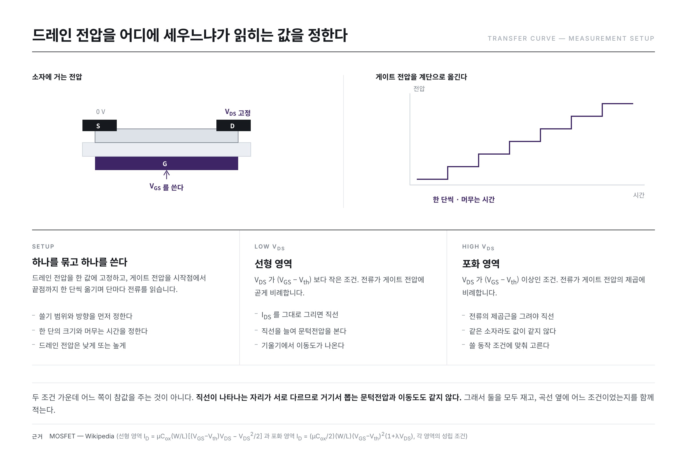
The procedure fits in one sentence. Fix the drain voltage at one value, move the gate voltage one step at a time from the starting point to the end point, and record the drain current at every step.

There is one choice to make here: at what value to fix the drain voltage. There are two answers, and both are used.

Fix it low — the transfer curve in the linear region

The Wikipedia article "MOSFET" writes the drain current for the case where V_GS is larger than the threshold voltage V_th and V_DS is smaller than (V_GS − V_th) as follows.

I_D = μ C_ox (W/L) [ (V_GS − V_th) V_DS − V_DS²/2 ]

Here μ is the mobility, C_ox the gate insulator capacitance per unit area, and W and L the width and length of the channel. Take V_DS very small and the V_DS²/2 term all but vanishes, leaving

I_D ≈ μ C_ox (W/L) V_DS × (V_GS − V_th)

behind. The only place the gate voltage appears is the last bracket. And so the current is directly proportional to the gate voltage. Plotted on a linear axis it gives a straight line, and extending that line to the left until it meets the horizontal axis lands near the threshold voltage.

Fix it high — the transfer curve in the saturation region

For the case where V_DS is at or above (V_GS − V_th), the "MOSFET" article writes

I_D = (μ C_ox / 2)(W/L)(V_GS − V_th)² (1 + λ V_DS)

The bracket enters squared. Set the trailing (1 + λ V_DS) aside for a moment and take the square root of both sides, and this becomes

√I_D = √( μ C_ox W / 2L ) × (V_GS − V_th)

so that this time it is not the current but the square root of the current that is directly proportional to the gate voltage.

Here lies the reason the two conditions tell us different things. At low V_DS the straight line appears only when I_D is plotted as it is; at high V_DS it appears only when √I_D is plotted. Since the straight line is found in a different place, the threshold voltage and mobility extracted from it are not the same either. Rather than one of them being the true value, the choice is made to match the operating condition under which the device will be used.

Why the vertical axis is laid out logarithmically

Now we plot the curve. And here a problem arises.

The currents of a device that is on and one that is off are not of comparable size. They are wildly different. The Wikipedia article "Organic field-effect transistor" puts the on/off current ratio, which expresses how well a device can be turned off, in the range 10⁶~10⁸. That is a million to a hundred million times.

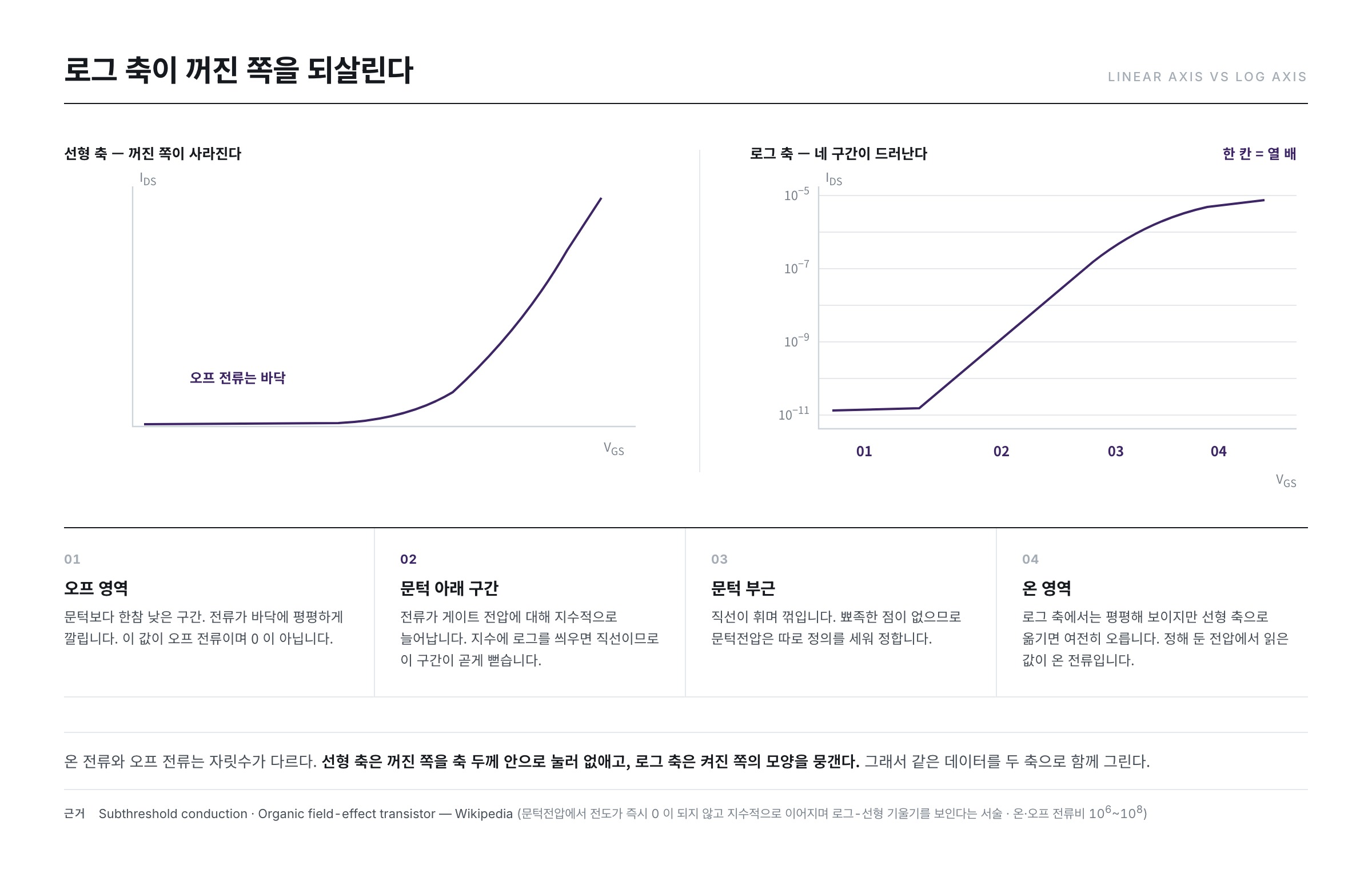
What happens on a linear vertical axis? The top of the scale has to be matched to the on current, so the off current, a millionth of it, disappears into the thickness of the axis. On the plot it shows only as a flat line hugging the bottom. Everything that happens on the off side is lost wholesale.

That is why a logarithm is applied to the vertical axis. On a logarithmic axis one division is a factor of ten. 10⁻¹¹ A and 10⁻³ A then sit side by side in the same picture, eight divisions apart. This is why transfer characteristics only begin to look like a transfer curve once they are moved onto a logarithmic axis.

In exchange, the logarithmic axis flattens the shape of the on side, because a doubling of the current moves only three tenths of a division. So both axes are drawn together. Overlay the same data once on a logarithmic axis and once on a linear axis, and the logarithmic axis takes charge of the off side while the linear axis takes charge of the on side.

The four regions of the curve

A transfer curve plotted on a logarithmic axis changes character four times as it runs from left to right.

The off region — only the leakage is left

This is the stretch where the gate voltage sits well below the threshold. The current lies almost flat along the bottom. This value is the off current I_off. What matters is that it is not zero.

The subthreshold region — the straight line on the logarithmic axis

This is the heart of the picture. The Wikipedia article "Subthreshold conduction" defines subthreshold conduction as the current that flows between source and drain when the gate-source voltage is below the threshold voltage, and states that it is also called subthreshold leakage.

The "Subthreshold conduction" article describes how conduction does not fall to zero the instant the threshold voltage is reached but continues exponentially with gate voltage. It further states that plotting this current against gate voltage produces a log-linear slope, which is called the subthreshold slope.

Apply a logarithm to an exponential function and you get a straight line. That is why this stretch runs straight on a logarithmic axis. The Wikipedia article "MOSFET" writes the current in this region as I_D ≈ I_D0 e^{(V_GS − V_th) / nV_T}. It has the same form as the one we met when looking at the diode in the previous series. The V_T in the denominator is the thermal voltage, and the "Thermal voltage" article puts it at about 25.85 mV at 300 K.

Why this region costs money and heat is also in the "Subthreshold conduction" article: as devices have shrunk, subthreshold conduction has become a large share of off-state leakage, and in some technology generations it can account for as much as 50% of total power consumption.

Near the threshold — there is no sharp point

This is the stretch where what was a straight line bends and turns over. The threshold voltage is fixed somewhere around here. There is, however, no sharp spot at which one can put a mark and say "the threshold is here." The curve merely bends smoothly. That is why a separate definition becomes necessary.

The on region — it keeps climbing after turning on

This is after the device is fully on. It looks almost flat on the logarithmic axis, but move to a linear axis and it is still climbing. The value read at a predetermined gate voltage is the on current I_on.

The values that come out of this one picture

Having named the four regions, let us first list the numbers extracted from this single picture. Each of them is treated separately in a later installment.

• Threshold voltage V_th — the gate voltage at which the device begins to turn on. It is fixed at the place where the curve bends.
• Subthreshold slope — how many mV of gate voltage it takes to raise the current tenfold. The unit is mV/decade.
• On current, off current and their ratio — the upper and lower ends of the curve, and the number of orders of magnitude between them.
• Mobility μ — obtained from the slope of the curve. How well the carriers run.
• Hysteresis — the mismatch between the curve measured going up and the curve measured coming down.

The subthreshold slope runs into a wall it cannot pass

The Wikipedia article "Subthreshold slope" writes this slope as follows.

S = ln(10) × (kT/q) × (1 + C_d/C_ox)

C_d is the depletion layer capacitance, C_ox the gate insulator capacitance, and kT/q the thermal voltage. Let us put the numbers in. At 300 K, kT/q is 25.85 mV and ln(10) is about 2.3026.

2.3026 × 25.85 mV ≈ 59.5 mV

This is the value when the bracket equals 1, that is, when C_d is close to 0 and the gate has full hold of the channel. This calculation is the basis on which the "Subthreshold slope" article gives 60 mV/decade at room temperature, 300 K as the smallest attainable value. However well a device is made, raising the current tenfold requires lifting the gate voltage by about 60 mV.

The bracket cannot fall below 1, because C_d/C_ox is always zero or greater. The "Subthreshold slope" article puts the representative measured value for scaled devices at about 70 mV/decade. Multiplying 59.5 mV by 1.2 gives 71.4 mV, which corresponds to a state in which C_d is about two tenths of C_ox.

Why this number matters becomes clear on multiplying it out. Suppose a device has a slope of 300 mV/decade; this article assumes that value for the sake of explanation. Climbing from the off state to an on current six orders of magnitude higher then requires a gate voltage of 300 mV × 6 = 1.8 V. With a slope of 100 mV/decade the same job takes 0.6 V. The supply voltage the circuit has to provide parts ways right here.

It is also worth noting that kT/q sits in the numerator. As the temperature rises, the wall itself rises with it.

Mobility comes out of the slope

Differentiating the linear-region equation set up earlier with respect to gate voltage gives

g_m = ∂I_D / ∂V_GS = μ C_ox (W/L) V_DS

which is the very quantity the Wikipedia article "MOSFET" defines as the transconductance g_m = ∂I_D/∂V_GS. Rearranging the right-hand side to leave μ alone gives

μ = g_m / [ C_ox (W/L) V_DS ]

and that is all. With nothing more than the slope of the curve and the dimensions of the device, the mobility comes out. Under saturation conditions the slope of the √I_D straight line seen earlier is used in the same way. Here too is a reason for measuring curves at both low V_DS and high V_DS. The procedure for actually extracting the value will be taken up separately in a later installment.

Sweep direction — going up is not the same as coming down

So far the gate voltage has been swept once, from low to high. What happens if we go all the way to the end and then measure once more on the way back down?

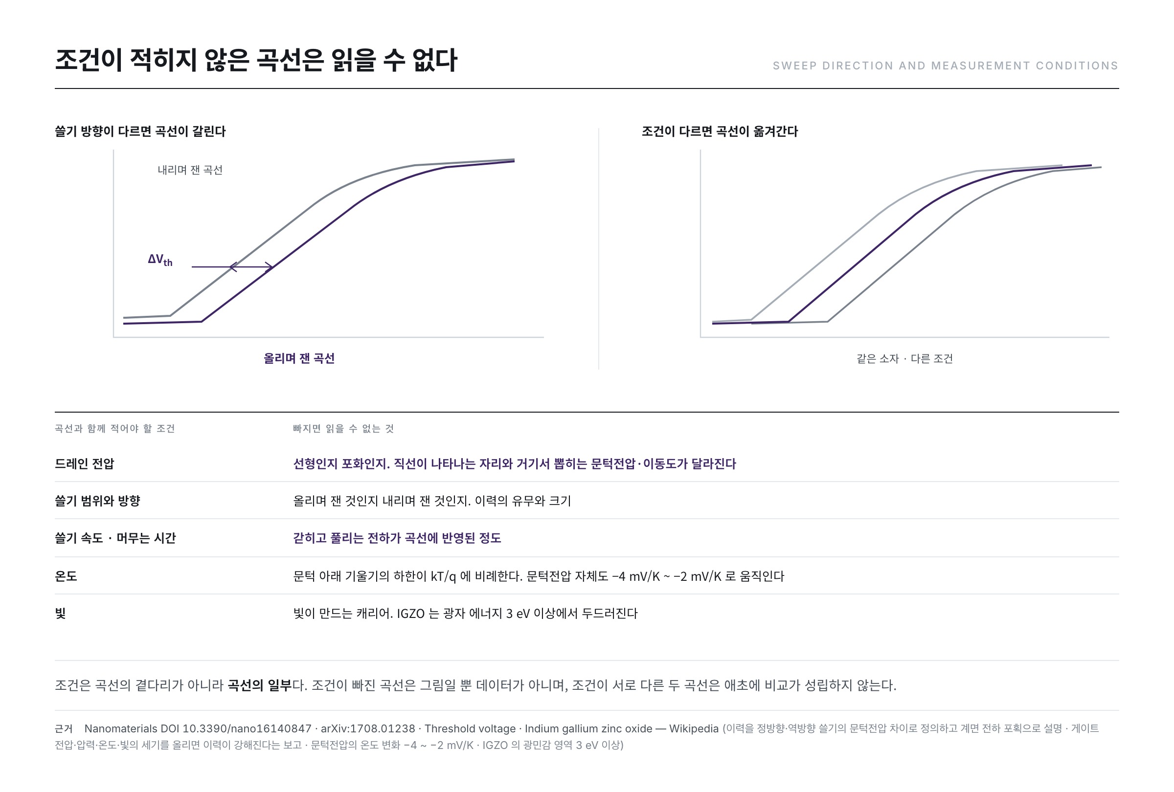
If the two curves lie on top of each other, nothing of what has just passed has been left behind in the device. If they do not, something has. This mismatch is called hysteresis.

A paper on hysteresis in carbon nanotube thin-film transistors (DOI 10.3390/nano16140847) defines gate-induced hysteresis as the difference between the threshold voltages obtained from the upward sweep and the downward sweep. The Nanomaterials paper explains its origin in terms of charge trapped at various interfaces, and states that adsorbed oxygen and water molecules play an important role.

The principle alone runs as follows. While the gate voltage is being raised, some of the carriers called into the channel are caught by defects where the insulator meets the semiconductor. Trapped charge cancels part of the electric field the gate has created. So on the way back down the channel is in a different state than before at the same gate voltage, and it looks as though the threshold voltage has shifted.

Being caught and being released both take time. Therefore how fast the sweep is run changes the result. Dwell longer at each point before reading and more of the trapping and releasing is reflected in the measurement. Under which conditions this hysteresis grows and what it tells us will be taken up separately in another series, on reliability.

A curve without its conditions written down cannot be read

Come this far and the final rule follows of its own accord. A transfer curve has meaning only as a package with its measurement conditions. The reasons have all appeared already.

• Drain voltage — whether it was taken low or high changes where the straight line appears, and with it the threshold voltage and mobility extracted there.
• Sweep range and direction — where the sweep starts and how far it goes, and whether it is on the way up or the way down, makes the two curves diverge.
• Sweep speed and dwell time — how long one waits at each point before reading the current changes how much of the trapping and releasing is reflected.
• Temperature — kT/q sits in the numerator of the subthreshold slope. The Wikipedia article "Threshold voltage" states that the threshold voltage itself varies with temperature between −4 mV/K and −2 mV/K, depending on the doping concentration.
• Light — a semiconductor makes carriers when light falls on it. The Wikipedia article "Indium gallium zinc oxide" states that IGZO transistors are somewhat photosensitive and that the effect is pronounced from deep violet into the ultraviolet, at photon energies above 3 eV.

That temperature and light really do move the curve is confirmed in the literature. An arXiv paper on hysteresis in molybdenum disulfide transistors (1708.01238) reports that raising any of gate voltage, pressure, temperature or light intensity strengthens the hysteresis.

So alongside the curve there must be written the V_DS value, the sweep range and direction, the step size, the measurement speed, the temperature, and whether there was light. A curve missing these is a picture, not data. All the more so for anyone trying to compare two devices, since if the conditions differ the comparison does not hold up at all.

Summary

• The transfer curve is obtained by fixing V_DS and sweeping V_GS. At low V_DS it is I_D, and at high V_DS it is √I_D, that is directly proportional to the gate voltage.
• The on and off currents differ in order of magnitude, so the vertical axis is drawn logarithmically. To see the shape of the on side, a linear axis is kept alongside it.
• The curve divides into four regions: off, subthreshold, near-threshold and on. The subthreshold region is an exponential function and therefore a straight line on a logarithmic axis.
• The subthreshold slope has a floor of about 60 mV/decade at room temperature, a value that comes out of ln(10) × 25.85 mV ≈ 59.5 mV.
• This one picture yields the threshold voltage, the slope, the on and off currents, the mobility and the hysteresis. In exchange, change the conditions and the same device gives a different curve.

The next installment takes the first item on this list. We look at how the threshold voltage is fixed as a single number on a curve that has no sharp point.

References

• MOSFET — Wikipedia : the drain-current equations for the linear, saturation and subthreshold regions together with the condition under which each holds, and the definition of the transconductance g_m = ∂I_D/∂V_GS
• Subthreshold conduction — Wikipedia : the definition of subthreshold conduction (the current flowing between source and drain at gate voltages below the threshold voltage), the account that conduction does not become zero at the threshold voltage but continues exponentially, the definition of the log-linear slope as the subthreshold slope, and the statement that off-state leakage can account for as much as 50% of total power consumption
• Subthreshold slope — Wikipedia : S = ln(10)·(kT/q)·(1 + C_d/C_ox), the minimum value of 60 mV/decade at room temperature, 300 K, and the representative measured value of about 70 mV/decade for scaled devices
• Threshold voltage — Wikipedia : the definition of the threshold voltage (the minimum gate-source voltage needed to create a conducting path between source and drain), the account that subthreshold leakage varies exponentially with gate bias, and the temperature variation of the threshold voltage, −4 mV/K ~ −2 mV/K
• Thermal voltage — Wikipedia : the definition V_T = kT/q and the value of about 25.85 mV at 300 K
• Organic field-effect transistor — Wikipedia : the on/off current ratio of 10⁶~10⁸, which expresses how well a device can be turned off
• Indium gallium zinc oxide — Wikipedia : the account that IGZO transistors are somewhat photosensitive and that the effect is pronounced from deep violet into the ultraviolet, at photon energies above 3 eV
• Hysteresis-Induced Performance Variations and Interfacial Charge Trapping Characteristics in Carbon Nanotube Thin-Film Transistors, Nanomaterials (DOI 10.3390/nano16140847) : the description of gate-induced hysteresis as the difference between the threshold voltages obtained from the forward and reverse sweeps, and the account explaining its origin in interfacial charge trapping and adsorbed oxygen and water molecules
• Hysteresis in the transfer characteristics of MoS₂ transistors (arXiv:1708.01238) : the report that raising any of gate voltage, pressure, temperature or light intensity strengthens the hysteresis
• ※ Passages quoted from the Wikipedia articles in the list above are under the CC BY-SA 4.0 license.