In the two previous installments we drew two curves. One is the output curve, obtained by tying the gate voltage to a single value and recording the current while sweeping the drain voltage. The other is the transfer curve, obtained by tying the drain voltage down and recording while sweeping the gate voltage.
Both curves are collections of points. Measure in steps of 0.01 V and several thousand points pile up. Yet what actually changes hands when a device is described is not several thousand points but a handful of numbers — the threshold voltage, the mobility, the off current and the like.
And here a problem arises. Nowhere on the curve is it written that “this point is the threshold voltage.” The curve merely bends smoothly. So in order to pull out a single number, one must first agree on where and how to read. That agreement is what a parameter is.
The operating values in this text are examples chosen to show the calculation, not the specifications of any particular company. Every figure quoted has been verified in the public literature, and the sources are listed at the end.
A parameter is not a measured value but a defined one
Take the threshold voltage as an example. The Wikipedia article “Threshold voltage” defines it as the minimum gate–source voltage needed to create a path along which current flows between source and drain. In words it is clear enough.
But the “Threshold voltage” article immediately attaches a proviso. Even when the gate voltage is below the threshold, current does flow. It is merely small, and it varies exponentially with gate voltage. That was the reason for using a logarithmic axis in the previous installment.
That makes the phrase “the voltage at which current begins to flow” awkward. Current was flowing from the start, so there is no point at all at which something not flowing begins to flow.
So the “Threshold voltage” article describes the practice actually used — a component datasheet fixes a measurable amount of current, such as 250 μA or 1 mA, and specifies the gate voltage that reaches that current as the threshold voltage.
The threshold voltage is not a value read out of the device but a value people have fixed by saying “let us count it as on once this much flows.” Change that number from 250 μA to 1 mA and the threshold voltage rises without anyone laying a finger on the device.
This is the central claim of this installment. A parameter is not a measured value but a defined one. Measurement takes us as far as the curve; the number is made by the definition.
One threshold voltage, several definitions
If there were only one definition there would be no confusion even so. But there is not just one.
The review paper published by Ortiz-Conde and colleagues in 2002 gathers and compares methods of extracting the threshold voltage, and it treats 11 methods drawn from linear-region transfer characteristics alone, plus 2 for the saturation region and 1 for amorphous thin-film devices. That amounts to 14 yardsticks for a single quantity. We will look at just three of them, the ones with the most distinct characters.
The constant-current method — draw one reference line
The gate voltage at which the current reaches a predetermined value is taken as the threshold voltage. This is the datasheet practice seen above. The review by Ortiz-Conde and colleagues makes clear that the current used by this method is a value fixed arbitrarily.
The assumption runs as follows — “we can agree in advance on the amount of current that separates on from off.” The calculation is simple and easy to automate. In exchange, change the agreed number and the result changes with it.
Linear extrapolation — lay a ruler on the steepest place
The transfer curve is plotted on a linear axis and a tangent is drawn at the point of greatest slope. The threshold voltage is taken as the gate voltage at which that tangent meets zero current, minus half the drain voltage.
The “slope” here is precisely the transconductance. The Wikipedia article “Transconductance” defines it as the change in output current divided by the change in input voltage and gives its unit as the siemens (S). It is the grip the gate has on the current.
The assumption runs as follows — “after turning on, the current is proportional to the gate voltage along a straight line, and extending that line backward gives the point at which it began to turn on.” For an ideal device that is true. In a real device the mobility falls as the voltage rises, so the curve departs from the straight line, and the result moves according to which point the ruler is laid on.
The second-derivative method — find where it bends
The current is differentiated twice with respect to gate voltage, and the voltage at which that value is greatest is taken as the threshold voltage.
The assumption runs as follows — “turning on is a bend in the curve, and the place where the bend is sharpest is that point.” If the current were zero below the threshold and proportional to the voltage above it, the first derivative would be a step and the second derivative a sharp peak standing where that step rises. In a real device the step is rounded off, but the peak remains. In exchange, differentiating twice greatly amplifies the measurement noise.
Laying three yardsticks on the same curve
Let us calculate directly how far they part. This article assumes the following model and values for its calculation.
- Transfer curve model — ID = K · nVT · ln(1 + e(VG − Vth0) / nVT) ÷ (1 + θ(VG − Vth0))
- This expression becomes an exponential curve below the threshold and approaches a straight line above it, with the θ term carrying the share by which the mobility falls.
- K = 1.0 × 10⁻⁵ A/V · n = 1.4 · VT = 0.0259 V (room-temperature thermal voltage) · Vth0 = 1.000 V · θ = 0.30 V−1 · VDS = 0.1 V · W/L = 10
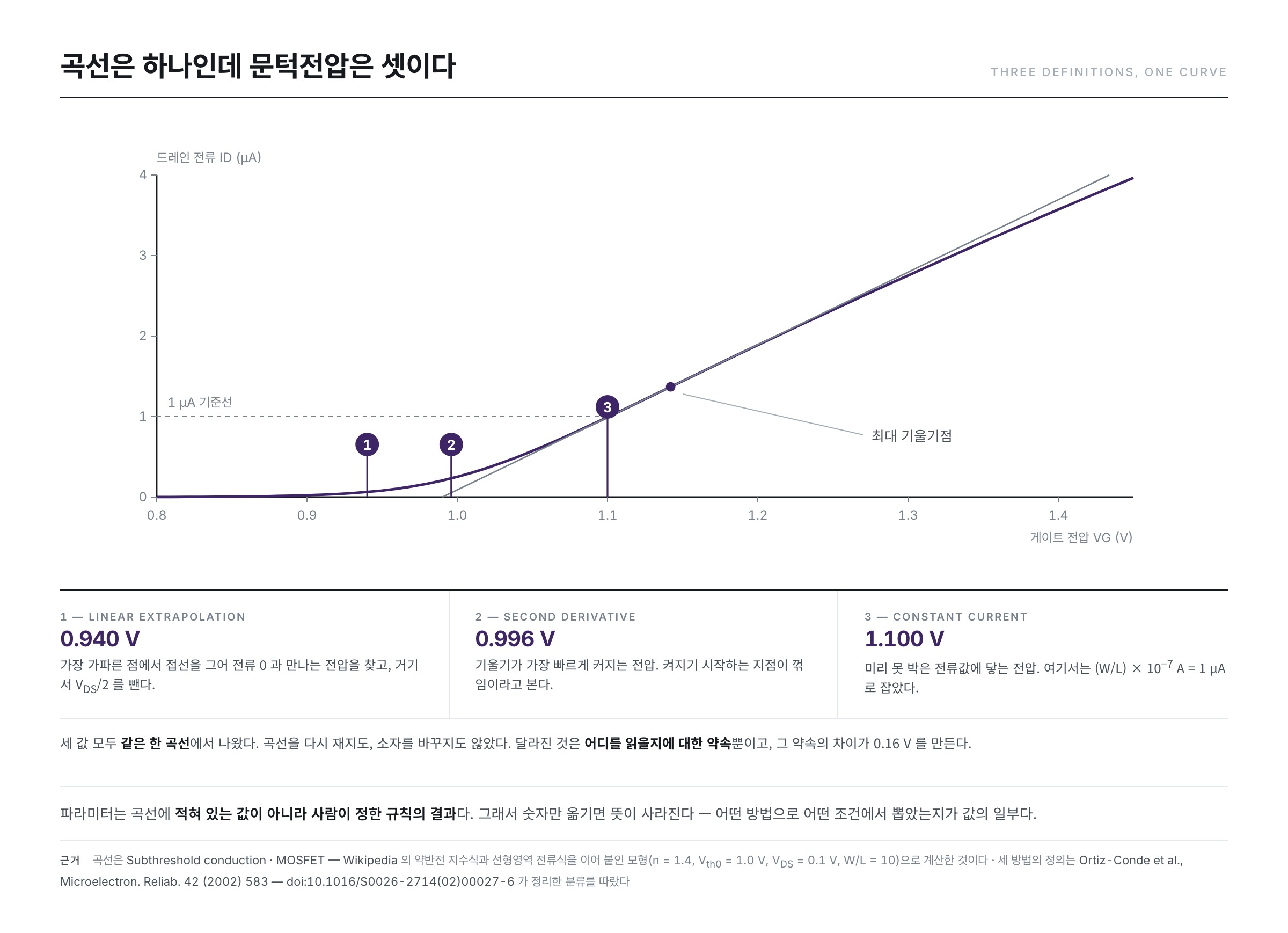
The “true value” written into the model is 1.000 V. Now we lay the three methods on this single curve.
- Linear extrapolation — the point of greatest slope is VG = 1.142 V, and the zero-current intercept of its tangent is 0.990 V. Subtracting VDS/2 = 0.05 V from this gives 0.940 V.
- Second-derivative method — the voltage at which the second derivative is greatest is 0.996 V.
- Constant-current method — taking the reference as (W/L) × 10−7 A = 1 μA gives 1.100 V.
It is the same curve. Nothing was measured again and no device was swapped. Yet the lowest value and the highest part by 0.160 V. The one closest to the true value is the second-derivative method, but that is because this model has a bend in it, not because the method is always right.
And so a parameter travels with its method and conditions
The measurement conditions change the value too. In the previous installment we said that the shape of a transfer curve depends on the value at which the drain voltage is tied down, and the threshold voltage is no different. Makris and Bucher, in their 2021 paper, point to this state of affairs in their opening paragraph — threshold voltage extraction methods that cover the full range of drain voltage with one yardstick are rare, and the reason is that the existing methods were built by looking at only a particular stretch of the curve. A yardstick made in the linear region does not fit when applied as it stands to the saturation region.
Having compared several methods on the same device, the paper by Makris and Bucher reports that the way the threshold voltage moves with the drain voltage differs from method to method. With some methods the value wavers when leaving saturation; with others it is nearly constant.
One conclusion comes out of this. A parameter whose extraction method and measurement conditions are not stated is merely a number, not information. Nor is it a comparison to set two numbers obtained by different methods side by side and argue over which is larger. When 0.940 and 1.100 come out of one and the same curve, what could possibly be said by holding one device's 0.94 against another's 1.10?
The map of parameters held in a single curve
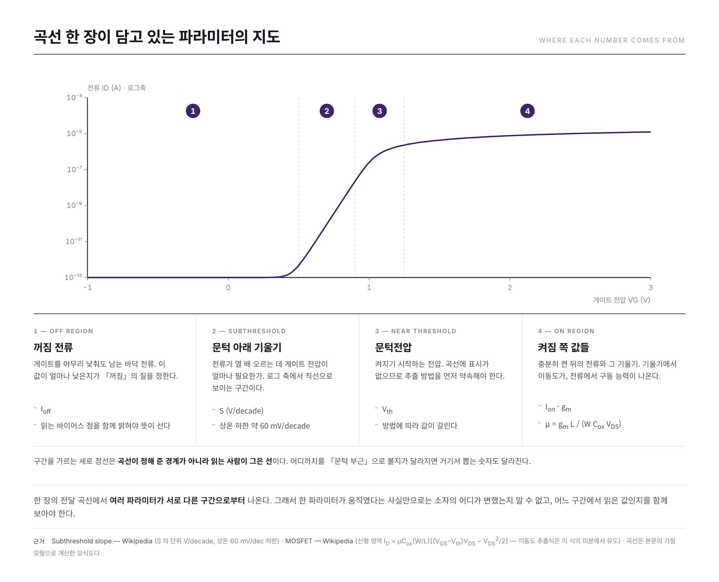
It is not only the threshold voltage that behaves this way. A single transfer curve yields several parameters, and they come from different stretches of it.
The off region — the off current
This is the side where the gate has been lowered far enough. The floor current that remains here is the off current. More than the value itself, at which gate voltage it was read must accompany it for the figure to mean anything.
The subthreshold region — the slope
This is the stretch that looks almost straight on a logarithmic axis. The value obtained here is the subthreshold slope (S). The Wikipedia article “Subthreshold slope” uses it as the gate voltage needed to raise the current tenfold, gives the unit as V/decade, and states that a decade here is a tenfold change in current. The “Subthreshold slope” article puts the theoretical floor at 60 mV/decade at room temperature, 300 K.
Calculated with the model assumed above, the slope of this stretch is 84 mV/decade, which agrees with the theoretical value the model carries, ln10 × n × kT/q = 2.303 × 1.4 × 0.0259 V = 83.5 mV/decade. Here n is the factor expressing how directly the gate holds the channel potential, and the closer it is to 1 the steeper the slope becomes.
Near the threshold — the threshold voltage
Exactly as seen above. It is only in this stretch that the definitions split into several.
The on region — the on current and the mobility
This is the side that has been turned fully on. The size of the current is itself the drive capability, and the mobility comes out of the slope of the current. We start from the linear-region current equation carried in the Wikipedia article “MOSFET.”
ID = μ Cox (W/L) [ (VGS − Vth) VDS − VDS2/2 ]
Take the drain voltage very small and the squared term at the back is negligible. Differentiate what remains with respect to gate voltage.
gm = ∂ID / ∂VGS = μ Cox (W/L) VDS
Solving for the mobility gives the following.
μ = gm L ÷ ( W Cox VDS )
Look at the right-hand side. Obtaining the mobility takes more than the slope alone: one must know the channel width W, the channel length L, the gate capacitance per unit area Cox and the drain voltage VDS, all of them. Let any one of the four differ and a different value comes out. The mobility, too, is not a measured value but a computed one.
Does the same value come out again — repeatability and reproducibility
Fixing the definition is not the end of it. For a number extracted by that definition to be of use, doing it again must give the same value. Let us split this into two branches.
The Wikipedia article “Repeatability” defines repeatability as how close successive measurements made under the same measurement conditions are to one another, and lists what goes into those “same conditions” — the same experimental tools, the same observer, the same measuring instrument used under the same conditions, the same location, and repetition within a short period. If ten measurements of the same device on the same instrument this morning do not scatter, there is repeatability.
The Wikipedia article “Reproducibility” uses reproducibility as reaching the same result when an independent, different research group does it again. The “Reproducibility” article also records the narrower sense used in interlaboratory experiments — the standard deviation of the difference between two measurements obtained in different laboratories is called the reproducibility. If repeatability is the scatter inside one laboratory, reproducibility is the scatter across laboratories.
Why both are needed follows directly from the earlier discussion. Repeatability is a matter of instruments and devices. If a contact wavers or the temperature changes, values scatter even on the same device. But reproducibility is a matter of definition. If one side obtains 0.940 V by linear extrapolation while the other obtains 1.100 V by the constant-current method, then however accurate the instruments are, reproducibility does not hold. It is not that the devices differ but that the yardsticks differ.
That is why, when parameters change hands, the extraction method and the measurement conditions are attached in front of the number. That is not a formality but a precondition of reproducibility.
The dimensions change the value — W and L
The current equation written earlier had (W/L) multiplied into it. W is the width of the channel and L its length. Compared to a waterway, they are its breadth and its length. The wider it is the more flows, and the longer it is the less flows, so the current is broadly proportional to W/L. The saturation-region equation is the same.
ID = (μn Cox / 2) (W/L) [ VGS − Vth ]2 [ 1 + λ VDS ]
The dimensions enter only as the single lump W/L. So to strip out the share belonging to the dimensions, all one has to do is divide the current by W/L.
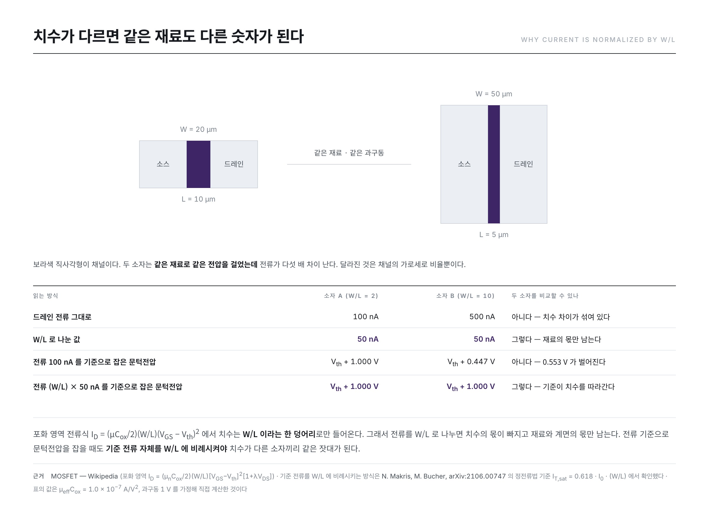
Let us see it in numbers. This article assumes μeffCox = 1.0 × 10⁻⁷ A/V2 and an overdrive voltage (VGS − Vth) = 1 V, and calculates in the saturation region.
- Device A — W = 20 μm and L = 10 μm, so W/L = 2. ID = (10−7/2) × 2 × 12 = 100 nA
- Device B — W = 50 μm and L = 5 μm, so W/L = 10. ID = (10−7/2) × 10 × 12 = 500 nA
- Divide the currents by W/L and both give 50 nA.
Same material, same voltage, and yet the currents differ fivefold. Divide them out and that difference disappears, leaving only the share belonging to the material and the interface.
Leave this normalization out and the definition itself collapses. Taking as an example the constant-current method with its reference current fixed at 100 nA, let us invert the saturation-region equation and find the overdrive voltage.
VGS − Vth = √( 2 ID ÷ ( μ Cox (W/L) ) )
- Device A — √(2 × 10⁻⁷ ÷ (10−7 × 2)) = √1.0 = 1.000 V
- Device B — √(2 × 10⁻⁷ ÷ (10−7 × 10)) = √0.2 = 0.447 V
Even if the two devices have the same threshold voltage, the values read off part by as much as 0.553 V. It is not that the devices differ but that the reference failed to follow the dimensions.
Let us change the reference current to (W/L) × 50 nA. The reference becomes 100 nA for device A and 500 nA for device B.
- Device A — √(2 × 10⁻⁷ ÷ (10−7 × 2)) = 1.000 V
- Device B — √(2 × 5 × 10−7 ÷ (10−7 × 10)) = 1.000 V
They come out the same. This is why the reference for the constant-current method in the earlier figure was written as (W/L) × 10−7 A. The paper by Makris and Bucher likewise writes the reference for the constant-current method as IT = 0.618 · I0 · (W/L), a form proportional to W/L. Only when the yardstick follows the dimensions does it become the same yardstick for devices of differing dimensions.
Summary
- A curve carries no mark saying “here is that value.” A parameter is not a measured value but a defined one, and measurement takes us only as far as the curve.
- Even one threshold voltage has several definitions. Laying linear extrapolation, the second-derivative method and the constant-current method on the same curve gives 0.940 V, 0.996 V and 1.100 V. A parameter must therefore travel carrying its extraction method and measurement conditions, and setting two numbers from different methods against each other is no comparison.
- A single curve yields a different parameter in each stretch — the off current on the off side, the slope (V/decade) below the threshold, the threshold voltage near the threshold, and the on current and mobility on the on side.
- Repeatability is getting the same value on measuring again under the same conditions; reproducibility is getting the same value on measuring somewhere else. Without fixing the definition, reproducibility cannot hold.
- The current is broadly proportional to W/L, so comparing devices of differing dimensions means looking at them divided by W/L. The reference current must be made proportional to W/L as well.
The next installment enters the middle cell of this map — it takes hold of the threshold voltage alone and looks at what makes that number move.
References
- Threshold voltage — Wikipedia : the definition of the threshold voltage (the minimum gate–source voltage that creates a conducting path), the account that current flows exponentially even below the threshold, and the account that datasheets specify the threshold voltage by a measurable amount of current such as 250 μA or 1 mA
- MOSFET — Wikipedia : the drain-current equations for the linear and saturation regions (in both, the dimensions enter as the single lump W/L), and the definition of the overdrive voltage
- Transconductance — Wikipedia : the definition of the transconductance gm = ΔIout/ΔVin and its unit, the siemens (S)
- Subthreshold slope — Wikipedia : the unit V/decade and the account that a decade is a tenfold change in current, and the floor of 60 mV/decade at room temperature, 300 K
- Repeatability — Wikipedia : the definition of repeatability and the list of “same conditions” (the same tools, observer, instrument and location, and repetition within a short period)
- Reproducibility — Wikipedia : the definition of reproducibility (reproduction by an independent, different research group), and the account that the standard deviation of the difference between two interlaboratory measurements is called the reproducibility
- A. Ortiz-Conde et al., “A review of recent MOSFET threshold voltage extraction methods”, Microelectronics Reliability 42 (2002) 583–596 : a review gathering and comparing 11 methods of extracting the threshold voltage from linear-region transfer characteristics, 2 for the saturation region and 1 for amorphous thin-film devices
- A. Ortiz-Conde, F. J. García-Sánchez, “Exploring MOSFET threshold voltage extraction methods”, IEEE EDS Distinguished Lecture, INAOE (2013) : lecture material by the authors of the review above; the account that the constant-current method uses an arbitrarily fixed current, the procedure of linear extrapolation (subtracting VD/2 from the intercept of the tangent at the maximum of the first derivative), and the grounds on which the second-derivative method uses the maximum of d2ID/dVG2
- N. Makris, M. Bucher, “On MOSFET Threshold Voltage Extraction Over the Full Range of Drain Voltage Based on Gm/ID”, arXiv:2106.00747 (2021) : the account that many existing extraction methods were built by looking at only a particular stretch of the curve, the comparison showing that the extracted threshold voltage moves differently with drain voltage from method to method, and the example setting the constant-current reference at IT = 0.618 · I0 · (W/L)
- ※ Passages quoted from the Wikipedia articles in the list above are under the CC BY-SA 4.0 license.